5.4: Method of Joints

The method of joints is a process used to solve for the unknown forces acting on members of a truss. As the name suggests, the method focuses on the joints or connection points between the members. While the method of sections discussed next is usually the fastest way to solve for the force in a specific member, the method of joints is usually the fastest way to solve for the unknown forces in all members of the truss.

Using the Method of Joints:

The method of joints and the method of sections both have the same initial steps, but will differ from one another once the external forces are found. The process used in the method of joints is outlined below:

To start, if the joints are not already labeled, we will begin by labeling all the joints with a letter. The exact order you label the joints in are not important, so long as you are consistent in your work. We will refer to joints by their letter (A, B, C...) and we will refer to the members by the two joints they connect (AB, AC, BC...). As a note, this text will always arrange the member names alphabetically, in order to avoid confusion (member AB, rather than member BA)

Figure \(\PageIndex{1}\): The first step in the method of joints is to label each joint and each member.

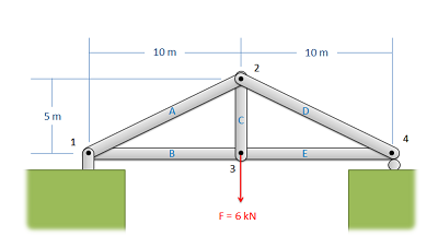
The second step is to solve for the external reaction forces supporting the truss. We can sometimes skip this step if the reaction forces are not necessary to solve for the internal forces, but when in doubt it is better to solve for the external reaction forces up front. To do this, treat the whole truss as a single rigid body. Draw a free body diagram of the truss, including the load forces and the external reaction forces supporting the truss, write out your equilibrium equations (sum of forces in the x, sum of forces in the y, and sum of moments), and finally solve the equilibrium equations for the unknown reaction forces.

Figure \(\PageIndex{2}\): Treat the entire truss as a rigid body and solve for the reaction forces supporting the truss structure.

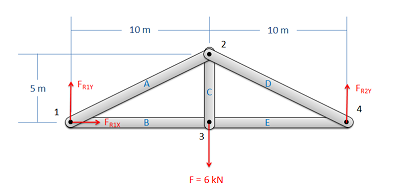
Next we get to the heart of the method of joints. We will assume there is a pin at each of the connection points between the members, and we will be drawing a free body diagram for each of those pins. We can do this one pin joint at a time, solving the equations as we go, or we can just draw all the free body diagrams at once and refer to those as we go. We will treat each of the pins as a particle for equilibrium analysis, and we will draw in the following forces.

• Any external reaction or load forces that may be acting at that joint. Add these as known values if you have already solved for them.
• One force for each two force member connected to that joint. Remember that for a two force member, the force will be acting along the line between the two connection points on the member. We will also need to guess if it will be a tensile or a compressive force. An incorrect guess now though will simply lead to a negative solution later on. A common strategy is to assume all member forces are tensile, then later in the solution any positive forces will be tensile forces and any negative forces will be compressive forces.

Be sure to label each force in your diagrams and include any known magnitudes and directions.

Figure \(\PageIndex{3}\): Drawing a free body diagram of each joint, we draw in the known forces as well as tensile forces from each two-force member.

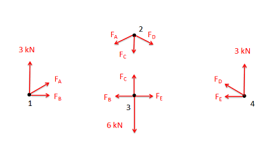
• Next we will write out the equilibrium equations for each of the joints. Since we treat the joints as particles, there will be force equations but no moment equations. We will have either two equations (for 2D problems) or three equations (for 3D problems) for each joint in the system. As the trusses get larger, so will the system of equations that we need to solve.
  • In planar trusses, the sum of the forces in the \(x\) direction will be zero and the sum of the forces in the \(y\) direction will be zero for each of the joints. \[ \sum \vec{F} = 0 \] \[ \sum F_x = 0 \, ; \,\,\, \sum F_y = 0 \]
  • In space trusses, the sum of the forces in the \(x\) direction will be zero, the sum of the forces in the \(y\) direction will be zero, and the sum of forces in the \(z\) direction will be zero for each of the joints. \[ \sum \vec{F} = 0 \] \[ \sum F_x = 0 \, ; \,\,\, \sum F_y = 0 \, ; \,\,\, \sum F_z = 0 \]

Finally, we will solve the equilibrium equations for the unknowns. If we are doing this by hand, we will want to work one joint at a time. Start at a joint with only two members connected (or three for 3D problems), and start by solving for the unknowns there. Once we have solved for those unknowns, we should be able to move to other nearby joints. If forces we already have solved for show up in these equations, we can use those values to solve for other unknowns. Just make sure when you pick the next joint you don't have more unknowns than available equations. Using this strategy, you can usually find a starting joint on one end of a truss, and work your way to the other end of the truss, solving for unknowns along the way.

Alternatively, if you have access to a computer, you can plug the equations into an equation solver and solve for all the unknowns at once. Though plugging all the equations into a computer may take more time, it may also save your significant time in instances where you need to fix errors in your equations or in your math.

Video lecture covering this section, delivered by Dr. Jacob Moore. YouTube source: https://youtu.be/B8SEG7xPI-o.

Example \(\PageIndex{1}\)

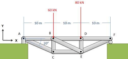
Find the force acting in each of the members in the truss bridge shown below. Remember to specify if each member is in tension or compression.

Figure \(\PageIndex{4}\): problem diagram for Example \(\PageIndex{1}\). A truss bridge represented as a 2D plane truss, with a standard-orientation \(xy\)-coordinate system.

Solution

Video \(\PageIndex{2}\): Worked solution to example problem \(\PageIndex{1}\), provided by Dr. Jacob Moore. YouTube source: https://youtu.be/vowewkEdTzw.

Example \(\PageIndex{2}\)

Find the force acting in each of the members of the truss shown below. Remember to specify if each member is in tension or compression.

Figure \(\PageIndex{5}\): problem diagram for Example \(\PageIndex{2}\). A plane truss mounted on a wall, with a standard-orientation \(xy\)-coordinate system.

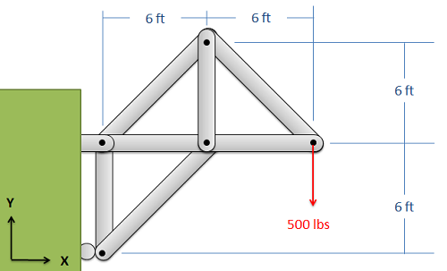
Solution

Video \(\PageIndex{3}\): Worked solution to example problem \(\PageIndex{2}\), provided by Dr. Jacob Moore. YouTube source: https://youtu.be/IxnClZ-ppjM.

Example \(\PageIndex{3}\)

Find the force acting in each of the members of the truss shown below. Remember to specify if each member is in tension or compression.

Figure \(\PageIndex{6}\): problem diagram for Example \(\PageIndex{3}\). A space truss supported by a single ball-and-socket joint, oriented on a 3D coordinate system with the \(yz\)-plane in the plane of the screen and the \(x\)-axis pointing out of the screen.

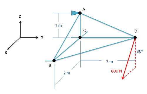
Solution

Video \(\PageIndex{4}\): Worked solution to example problem \(\PageIndex{3}\), provided by Dr. Jacob Moore. YouTube source: https://youtu.be/sDKESSbufEk.