
6.7: Belt Friction
- Page ID
- 53833

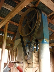
In any system where a belt or a cable is wrapped around a pulley or some other cylindrical surface, we have the potential for friction between the belt or cable and the surface it is in contact with. In some cases, such as a rope over a tree branch being used to lift an object, the friction forces represent a loss. In other cases such as a belt-driven system, these friction forces are put to use transferring power from one pulley to another pulley.

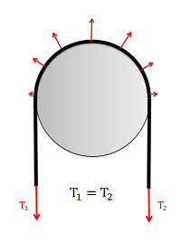
For analysis, we will start a flat, massless belt passing over a cylindrical surface. If we have an equal tension in each belt, the belt will experience a non-uniform normal force from the cylinder that is supporting it.
In a frictionless scenario, if we were to increase the tension on one side of the rope it would begin to slide across the cylinder. If friction exists between the rope and the surface though, the friction force will oppose with sliding motion, and prevent it up to a point.
Friction in Flat Belts
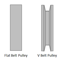
A flat belt is any system where the pulley or surface only interacts with the bottom surface of the belt or cable. If the belt or cable instead fits into a groove, then it is considered a V belt.
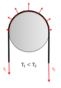
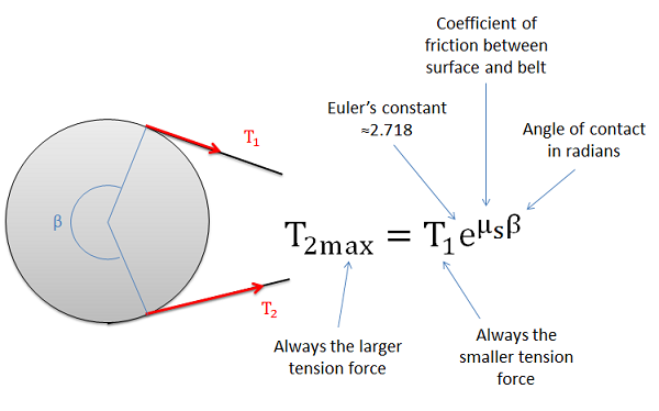
When analyzing systems with belts, we are usually interested in the range of values for the tension forces where the belt will not slip relative to the surface. Starting with the smaller tension force on one side \((T_1)\), we can increase the second tension force \((T_2)\) to some maximum value before slipping. For a flat belt, the maximum value for \(T_2\) will depend on the value of \(T_1\), the static coefficient of friction between the belt and the surface, and the contact angle between the belt and the surface \((\beta)\) given in radians, as described in the equation below.
\[T_{2_{max}} = T_1 \, e ^ {\mu_s \beta} \]
Friction in V Belts
A V belt is any belt that fits into a groove on a pulley or surface. For the V belt to be effective, the belt or cable will need to be in contact with the sides of the groove, but not the base of the groove as shown in the diagram below. With the normal forces on each side, the vertical components must add up the the same as what the flat belt would have, but the added horizontal components of the normal forces, which cancel each other out, increase the potential for friction forces.
The equation for the maximum difference in tensions in V belt systems is similar to the equation in flat belt systems, except we use an "enhanced" coefficient of friction that takes into account the increased normal and friction forces possible because of the groove.
\[ T_{2_{max}} = T_1 \ e ^{\mu_{s \ (enh)} \beta} , \,\, \text{ where} \]
\[ \mu_{s \ (enh)} = \frac{\mu_s}{ \sin \left( \frac{\alpha}{2} \right)} \]
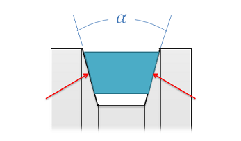
As we can see from the equation above, steeper sides to the groove (which would result in a smaller angle \(\alpha\)) result in an increased potential difference in the tension forces. The tradeoff with steeper sides, however, is that the belt becomes wedged in the groove and will require force to unwedge itself from the groove as it leaves the pulley. This will cause losses that decrease the efficiency of the belt driven system. If very high tension differences are required, chain-driven systems offer an alternative that is usually more efficient.
Torque and Power Transmission in Belt-Driven Systems
In belt-driven systems there is usually an input pulley and one or more output pulleys. To determine the maximum torque or power that can be transmitted by the belt, we will need to consider each of the pulleys independently, understanding that slipping occurring at either the input or the output will result in a failure of the power transmission.
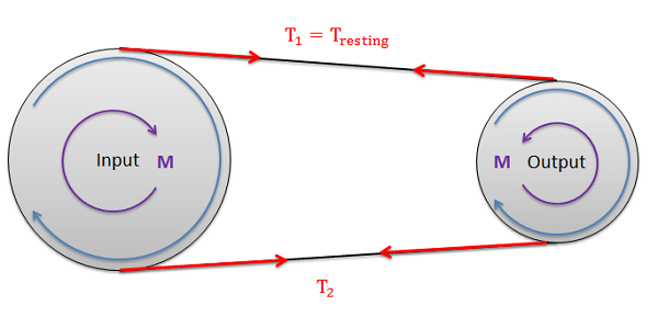
The first step in determining the maximum torque or power that can be transmitted in the belt drive is to determine the maximum possible value for \(T_2\) before slipping occurs at either the input or output pulley (again, slipping at either location cannot occur). To start we will often be given the "resting tension". This is the tension in the belt when everything is stationary and before power is transferred. Sometimes machines will have adjustments to increase or decrease the resting tension by slightly increasing or decreasing the distance between the pulleys. If we turn on the machine and increase the load torque at the output, the tension on one side of the pulleys will remain constant as the resting tension while the tension on the other side will increase. Since the resting tension is constant and is always the lower of the two tensions, it will be the \(T_1\) tension in equations \(\PageIndex{1}\) and \(\PageIndex{2}\).
Though it is often wise to check, assuming the pulleys are made of the same material (and therefore have the same coefficients of friction), it is often assumed that the belt will first slip at the smaller of the two pulleys in a single-input-single-output belt system. This is because the smaller pulley will have the smaller contact angle \((\beta)\), while all other values remain the same.
Once we have the maximum value for \(T_2\), we can use that to find the torque at the input pulley and the torque at the output pulley. Note that these two values will not be the same unless the pulleys are the same size. To find the torque, we will simply need to find the net moment exerted by the two tension forces, where the radius of the pulley is the moment arm.
Maximum input torque before slipping:\[ M_{max} = (T_{2_{max}} - T_1) (r_{input}) \]
Maximum output torque before slipping:\[ M_{max} = (T_{2_{max}} - T_1) (r_{output}) \]
To find the maximum power we can transfer with the belt drive system, we will use the rotational definition of power, where the power is equal to the torque times the angular velocity in radians per second. Unlike the torque, the power at the input and the output will be the same, assuming no inefficiencies.
\[ P_{max} = (M_{input \ max}) (\omega_{input}) = (M_{output \ max}) (\omega_{output}) \]
Example \(\PageIndex{1}\)
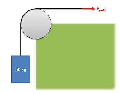
A steel cable supporting a 60-kg mass is run a quarter of the way around a steel cylinder and supported by a pulling force as shown in the diagram below. The static coefficient of friction between the cable and the steel cylinder is 0.3.
- What is the minimum pulling force required to lift the mass?
- What is the minimum pulling force required to keep the mass from falling?
- Solution
-
Video \(\PageIndex{2}\): Worked solution to example problem \(\PageIndex{2}\), provided by Dr. Jacob Moore. YouTube source: https://youtu.be/SXtKkoF4xtc.
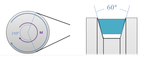
Example \(\PageIndex{2}\)
A V-belt pulley as shown below is used to transmit a torque. If the diameter of the pulley below is 5 inches, the resting tension in the belt is 20 lbs, and the coefficient of friction between the belt material and the pulley is 0.4, what is the maximum torque the pulley can exert before slipping?
- Solution
-
Video \(\PageIndex{3}\): Worked solution to example problem \(\PageIndex{2}\), provided by Dr. Jacob Moore. YouTube source: https://youtu.be/RLZxKEJVLeo.
Example \(\PageIndex{3}\)
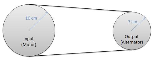
A flat belt is being used to transfer power from a motor to an alternator as shown in the diagram below. The coefficient of friction between the belt material and the pulley is 0.5. If we require a power of 100 Watts (Nm/s) while the input is rotating at a rate of 1000 rpm and the output is rotating at a rate of 1428.6 rpm, what is the required resting tension in the belt? (Assume contact angles of approximately 180 degrees)
- Solution
-
Video \(\PageIndex{4}\): Worked solution to example problem \(\PageIndex{3}\), provided by Dr. Jacob Moore. YouTube source: https://youtu.be/K7PhVhXgqUQ.