7.5: Two-Dimensional Motion with Polar Coordinates

Last updated
Save as PDF

Page ID: 53926

\( \newcommand{\vecs}[1]{\overset { \scriptstyle \rightharpoonup} {\mathbf{#1}} } \) \( \newcommand{\vecd}[1]{\overset{-\!-\!\rightharpoonup}{\vphantom{a}\smash {#1}}} \)\(\newcommand{\id}{\mathrm{id}}\) \( \newcommand{\Span}{\mathrm{span}}\) \( \newcommand{\kernel}{\mathrm{null}\,}\) \( \newcommand{\range}{\mathrm{range}\,}\) \( \newcommand{\RealPart}{\mathrm{Re}}\) \( \newcommand{\ImaginaryPart}{\mathrm{Im}}\) \( \newcommand{\Argument}{\mathrm{Arg}}\) \( \newcommand{\norm}[1]{\| #1 \|}\) \( \newcommand{\inner}[2]{\langle #1, #2 \rangle}\) \( \newcommand{\Span}{\mathrm{span}}\) \(\newcommand{\id}{\mathrm{id}}\) \( \newcommand{\Span}{\mathrm{span}}\) \( \newcommand{\kernel}{\mathrm{null}\,}\) \( \newcommand{\range}{\mathrm{range}\,}\) \( \newcommand{\RealPart}{\mathrm{Re}}\) \( \newcommand{\ImaginaryPart}{\mathrm{Im}}\) \( \newcommand{\Argument}{\mathrm{Arg}}\) \( \newcommand{\norm}[1]{\| #1 \|}\) \( \newcommand{\inner}[2]{\langle #1, #2 \rangle}\) \( \newcommand{\Span}{\mathrm{span}}\)\(\newcommand{\AA}{\unicode[.8,0]{x212B}}\)

Two-dimensional motion (also called planar motion) is any motion in which the objects being analyzed stay in a single plane. When analyzing such motion, we must first decide the type of coordinate system we wish to use. The most common options in engineering are rectangular coordinate systems, normal-tangential coordinate systems, and polar coordinate systems. Any planar motion can potentially be described with any of the three systems, though each choice has potential advantages and disadvantages.

The polar coordinate system uses a distance \((r)\) and an angle \((\theta)\) to locate a particle in space. The origin point will be a fixed point in space, but the \(r\)-axis of the coordinate system will rotate so that it is always pointed towards the body in the system. The variable \(r\) is also used to indicate the distance from the origin point to the particle. The theta-axis will then be 90 degrees counterclockwise from the \(r\)-axis with the variable \(\theta\) being used to show the angle between the \(r\)-axis and some fixed axis that does not rotate. The diagram below shows a particle with a polar coordinate system.

A particle is in the first quadrant of a Cartesian plane, with the vector r pointing from the origin to its position and making an angle of theta with the x-axis. At the origin, a unit vector u-hat_r points in the direction of the vector r, and the vector u-hat_theta points 90 degrees counterclockwise from u-hat_r. — Figure \(\PageIndex{1}\): In the polar coordinate system, the \(r\) direction always points from the origin point to the body. The variable \(r\) is also used to indicate the distance between the two points. The theta direction will always be 90° counterclockwise from the \(r\) direction. Theta is also used to indicate the angle between the \(r\) direction and some fixed axis used for reference. The \(\hat{u}_r\) and \(\hat{u}_{\theta}\) vectors represent unit vectors in the \(r\) and \(\theta\) directions, respectively.

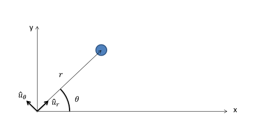
Polar coordinate systems work best in systems where a body is being tracked via a distance and an angle, such as a radar system tracking a plane. In cases such as this, the raw data from this in the form of an angle and a distance would be direct measures of \(\theta\) and \(r\) respectively. Polar coordinate systems will also serve as the base for extended body motion, where motors and actuators can directly control things like \(r\) and \(\theta\).

The way the coordinate system is defined, the \(r\)-axis will always point from the origin point to the body. The distance from the origin to the point is defined as \(r\) with no component of the position being in the \(\theta\) direction.

\[ \text{Position:} \quad \, r_{p/o}(t) = r \hat{u}_r + 0 \ \hat{u}_{\theta} \]

To find the velocity, we need to take the derivative of the position function over time. Since the distance \(r\) can change over time as well as the direction \(\hat{u}_r\) changing over time to track the body, we need to worry about the derivative of \(r\) as well as the derivative of the unit vector. Like we did with the normal-tangential systems, we will use the product rule and then substitute in a value for the derivative of the unit vector.

\[ \text{Velocity:} \quad \, v(t) = \dot{r} \hat{u}_r + r \dot{\hat{u}}_r = \dot{r} \hat{u}_r + r \dot{\theta} \hat{u}_{\theta} \]

To find the acceleration, we need to take the derivative of the velocity function. As all of these terms, including the unit vectors, change over time, we will need to use the product rule extensively. The \(\hat{u}_r\) term will split into two terms, and the \(\hat{u}_{\theta}\) term will split into three terms.

\[ \text{Acceleration:} \quad \, a(t) = \ddot{r} \hat{u}_r + \dot{r} \dot{\hat{u}_r} + \dot{r} \dot{\theta} \hat{u}_{\theta} + r \ddot{\theta} \hat{u}_{\theta} + r \dot{\theta} \dot{\hat{u}}_{\theta} \]

Again we will need to substitute in values for the derivatives of the unit vectors similar to before, but it is worth mentioning that the derivative of the \(\hat{u}_{\theta}\) vector as it rotates counterclockwise is in the negative \(\hat{u}_r\) direction.

A particle on the polar coordinate system rotates counterclockwise by a small amount d theta. The vector u-hat_r points from the head of the initial r-direction unit vector to the final r-direction unit vector, and the vector u-hat_theta points from the head of the initial theta-direction unit vector to the final theta-direction unit vector. — Figure \(\PageIndex{2}\): The derivatives of the \(\hat{u}_r\) and \(\hat{u}_{\theta}\) unit vectors. Notice that the derivative of the \(\hat{u}_{\theta}\) vector is in the negative \(\hat{u}_r\) direction.

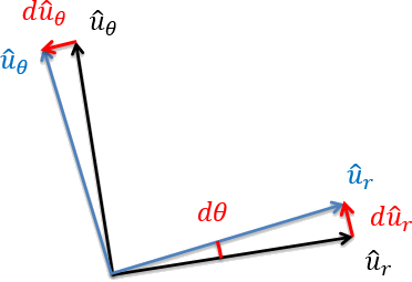
After substituting in the derivatives of the unit vectors and simplifying the function, we arrive at our final equation for the acceleration.

\begin{align} \text{Acceleration:} \quad \, a(t) &= \ddot{r} \hat{u}_r + \dot{r} \dot{\theta} \hat{u}_{\theta} + \dot{r} \dot{\theta} \hat{u}_{\theta} + r \ddot{\theta} \hat{u}_{\theta} - r \dot{\theta}^2 \hat{u}_r \\[5 pt] &= \left( \ddot{r} - r \dot{\theta}^2 \right) \hat{u}_r + \left( 2 \dot{r} \dot{\theta} + r \ddot{\theta} \right) \hat{u}_{\theta} \end{align}

Though this final equation has a number of terms, it is still just two components in vector form. Just as with the normal-tangential coordinate system, we will need to remember that we will need to split the single vector equation into two separate scalar equations. In this case we will have the equation for the terms in the \(r\) direction and the equation for the terms in the \(\theta\) direction.

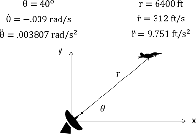
Video lecture covering this section, delivered by Dr. Jacob Moore. YouTube source: https://youtu.be/F4i0Kz660aE.

Example \(\PageIndex{1}\)

A radar tracking station gives the following raw data to a user at a given point in time. Based on this data, what is the current velocity and acceleration in the \(r\) and \(\theta\) directions? What is the current velocity and acceleration in the \(x\) and \(y\) directions?

An airplane located in the first quadrant of a Cartesian coordinate plane, with a radar tracking station at the origin. The polar-coordinate data of the plane's current position is given as theta = 40 degrees, theta-dot = -0.039 rad/s, theta double-dot = 0.003807 rad/s², r = 6400 ft, r-dot = 312 ft/s, and r double-dot = 9.751 ft/s². — Figure \(\PageIndex{3}\): Problem diagram for Example \(\PageIndex{1}\). The instantaneous polar-coordinate position values of an airplane are given as tracked by a radar station, as well as the first and second derivatives of these quantities.

Solution: Video \(\PageIndex{2}\): Worked solution to example problem \(\PageIndex{1}\), provided by Dr. Majid Chatsaz. YouTube source: https://youtu.be/HP4WiIa3Nc0.

Example \(\PageIndex{2}\)

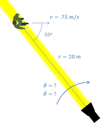
A spotlight is tracking an actor as he moves across the stage. If the actor is moving with a constant velocity as shown below, what values do we need for the spotlight angular velocity \((\dot{\theta})\) and spotlight angular acceleration \((\ddot{\theta})\) so that the spotlight remains fixed on the actor?

A top-down view of a stage with a spotlight in the lower right corner, its beam shining diagonally 20 meters across the stage on an actor in the upper left corner. The actor is moving horizontally at 0.75 m/s to the right, 55 degrees above the diagonal line of the spotlight beam. The spotlight is rotating clockwise to track the actor. — Figure \(\PageIndex{4}\): problem diagram for Example \(\PageIndex{2}\). A spotlight rotates to follow an actor moving across stage at a known velocity and starting from a known position in relation to the spotlight.

Solution: Video \(\PageIndex{3}\): Worked solution to example problem \(\PageIndex{2}\), provided by Dr. Majid Chatsaz. YouTube source: https://youtu.be/jyD1seNQI14.