7.7: Relative Motion Systems

Relative motion analysis is the analysis of bodies where more than one body is in motion and we are in some way examining the motion of one moving particle relative to another moving particle. An example would be cars on a highway. If you are in one of many cars moving down one side of the highway, you and the other cars will all have velocities in a single direction. From your perspective inside the car, though, fast cars in front of you will appear to be moving away from you and slow cars in front of you will appear to be moving towards you. By knowing your speed, and by observing how fast the cars are moving away from you or towards you, you could determine or at least estimate how fast these cars are going. The process of using your speed in conjunction with the relative velocities of the other cars to find the other cars' speed is relative motion analysis.

Relative Motion in One Dimension:

In a single dimension, we will usually have at least two moving particles as well as some fixed reference point. We usually call the fixed reference point \(O\), and then label the other points \(A\), \(B\), and so on. In the diagram, below we can see an example of this, with a fixed reference point at \(O\), a police car at \(A\), and a speeding car at \(B\).

Figure \(\PageIndex{1}\): In a single dimension we have a fixed reference point \(O\), as well as at least two moving bodies (labeled as \(A\) and \(B\) in this case). The \(r\) vectors represent the distances between bodies, with the subscript indicating the point we are observing and the point we are observing from. The subscripts should always have the following format: point being observed / point we are observing from.

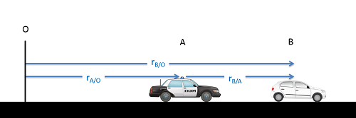
As we can see from the diagram above, the sum of the distance from \(O\) to \(A\) \((r_{A/O})\) and the distance from \(A\) to \(B\) \((r_{B/A})\) will be equal to the distance from \(O\) to \(B\) \((r_{B/O})\). This gives us our position equation below.

\[ \text{Position:} \quad \, r_{B/O} = r_{A/O} + r_{B/A} \]

One thing we should notice about the subscripts is that if we keep to our standard naming convention (point being observed / point we are observing from) then we should be able to see which points cancel out and which remain. In this case, the \(A\)'s on the top and bottom on the right cancel out, leaving just a \(B\) on the top and an \(O\) on the bottom. This matches the subscript on the left of the equation.

Furthermore, we can take the derivative of this equation to relate velocities, or a double derivative to relate accelerations. This means that if we know any two of the terms in the equations below, we can solve for the third.

\begin{align} \text{Velocity:} \quad &\, v_{B/O} = v_{A/O} + v_{B/A} \\[5pt] \text{Acceleration:} \quad &\, a_{B/O} = a_{A/O} + a_{B/A} \end{align}

Relative Motion in Two Dimension:

Just as with one dimension, we can start by examining a set of relative positions. In this case we will use the example of two planes moving through the sky. We may wish to deduce the position of plane B on a map, based on our observations from plane A. By using the information we have on our position relative to some set location, along with the relative position read in from on board instrumentation, we should be able to determine the absolute position (including an \(x\) and \(y\) coordinate) for plane B.

Figure \(\PageIndex{2}\): In two dimensions we have a fixed reference point \(O\), as well as at least two moving bodies (labeled as \(A\) and \(B\) in this case). The \(\vec{r}\) vectors represent the distance vectors between bodies, with the subscript indicating the starting and ending point. The subscripts should always be formatted end point / starting point.

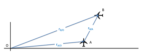
In two dimensions, we will use the same equations as before, except this time we will be using vectors rather than scalar values in our equations.

\begin{align} \text{Position:} \quad &\, \vec{r}_{B/O} = \vec{r}_{A/O} + \vec{r}_{B/A} \\[5pt] \text{Velocity:} \quad &\, \vec{v}_{B/O} = \vec{v}_{A/O} + \vec{v}_{B/A} \\[5pt] \text{Acceleration:} \quad &\, \vec{a}_{B/O} = \vec{a}_{A/O} + \vec{a}_{B/A} \end{align}

To solve these equations, we will almost always break the vector equations down into a set of component equations. This will let us solve these equations with simple algebra. Because we have more than one particle, we usually use rectangular coordinate systems for this with a universal set of \(x\) and \(y\) coordinates.

Video lecture covering this section, delivered by Dr. Jacob Moore. YouTube source: https://youtu.be/A5aJ2VYvwkw.

Example \(\PageIndex{1}\)

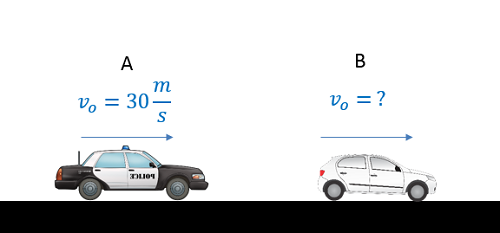
A police officer notices a car speeding by. If the police car is traveling 30 m/s and the radar gun measures the relative velocity to be 15 m/s, how fast is the speeding car actually going? If the police car immediately begins accelerating at a constant rate and catches up to the speeding car after 15 seconds, what is the rate of acceleration of the police car?

Figure \(\PageIndex{3}\): problem diagram for Example \(\PageIndex{1}\). A police car and a speeding car it is chasing after travel in the same direction on a straight road.

Solution

Video \(\PageIndex{2}\): Worked solution to example problem \(\PageIndex{1}\), provided by Dr. Majid Chatsaz. YouTube source: https://youtu.be/YndovN5yWfc.

Example \(\PageIndex{2}\)

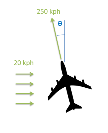
A plane has an airspeed of 250 kilometers per hour (airspeed is the velocity of the plane relative to the air) and is flying though an easterly crosswind with a speed of 20 kilometers per hour. If the plane wants to maintain a direct northerly course, what is the angle the plane must point into the wind \((\theta)\)?

Figure \(\PageIndex{4}\): problem diagram for Example \(\PageIndex{2}\). A plane aiming to fly directly northwards experiences easterly crosswinds.

Solution

Video \(\PageIndex{3}\): Worked solution to example problem \(\PageIndex{2}\), provided by Dr. Majid Chatsaz. YouTube source: https://youtu.be/ga1qcV38zYA.

Example \(\PageIndex{3}\)

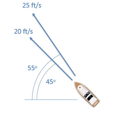
You are in a boat that is traveling through the water in an area of swift currents. One instrument measures your speed with respect to the water to be 20 ft/s with your boat pointed at a 45-degree angle. GPS, however, measures your absolute speed and direction to be 25 ft/s at a 55-degree angle. Based on this information, what is the speed and direction of the water current in this area?

Figure \(\PageIndex{5}\): problem diagram for Example \(\PageIndex{3}\). Instruments on a boat return different readings for its absolute velocity vs. its velocity relative to the surrounding water.

Solution

Video \(\PageIndex{4}\): Worked solution to example problem \(\PageIndex{3}\), provided by Dr. Majid Chatsaz. YouTube source: https://youtu.be/j8vnM_hrnQg.