8.3: Equations of Motion in Normal-Tangential Coordinates

Continuing our discussion of kinetics in two dimensions, we can examine Newton's Second Law as applied to the normal-tangential coordinate system. In its basic form, Newton's Second Law states that the sum of the forces on a body will be equal to the mass of that body times the rate of acceleration. For bodies in motion, we can write this relationship out as the equation of motion.

\[ \sum \vec{F} = m * \vec{a} \nonumber \]

Just as we did with with rectangular coordinates, we will break this single vector equation into two separate scalar equations. This involves identifying the normal and tangential directions and then using sines and cosines to break the given forces and accelerations down into components in those directions.

Figure \(\PageIndex{1}\): When working in the normal-tangential coordinate system, any given forces or accelerations can be broken down using sines and cosines as long as the angle of the force or acceleration is known relative to the normal and tangential directions.

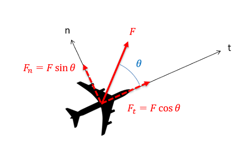
\begin{align} \sum F_n &= m * a_n \\[5pt] \sum F_t &= m * a_t \end{align}

Just as with rectangular coordinates, these equations of motion are often used in conjunction with the kinematics equations, which relate positions, velocities and accelerations as discussed in the previous chapter. In particular, we will often substitute the known values below for the normal and tangential components for acceleration.

\[ a_n = v * \dot{\theta} = \frac{v^2}{\rho} \]

\[ a_t = \dot{v} \]

Normal-tangential coordinates can be used in any kinetics problem; however, they work best with problems where forces maintain a consistent direction relative to some body in motion. Vehicles in motion are a good example of this: the direction of the forces applied are largely dependent on the current direction of the vehicle, and these forces will rotate with the vehicle as it turns.

Video lecture covering this section, delivered by Dr. Jacob Moore. YouTube source: https://youtu.be/PK2swJu37sg.

Example \(\PageIndex{1}\)

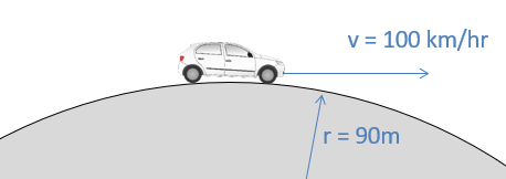
A 1000-kg car travels over a hill at a constant speed of 100 kilometers per hour. The top of the hill can be approximated as a circle with a 90-meter radius.

• What is the normal force the road exerts on the car as it crests the hill?
• How fast would the car have to be going to get airborne?

Figure \(\PageIndex{2}\): problem diagram for Example \(\PageIndex{1}\). A car is at the top of a hill, moving towards the right at a constant speed of 100 km/hr.

Solution

Video \(\PageIndex{2}\): Worked solution to example problem \(\PageIndex{1}\), provided by Dr. Majid Chatsaz. YouTube source: https://youtu.be/KOLdXpQ5M1Q.

Example \(\PageIndex{2}\)

A 2500-pound car is traveling 40 feet per second. The coefficient of friction between the car’s tires and the road is 0.9.

• If the car is maintaining a constant speed, what is the minimum radius of curvature before slipping?
• Assuming the car is speeding up at a rate of 10 ft/s², what is the minimum radius of curvature before slipping?

Figure \(\PageIndex{3}\): problem diagram for Example \(\PageIndex{2}\). A car travels around a circular path in a counterclockwise direction.

Solution

Video \(\PageIndex{3}\): Worked solution to example problem \(\PageIndex{2}\), provided by Dr. Majid Chatsaz. YouTube source: https://youtu.be/Gw0_H0wdqm8.

Example \(\PageIndex{3}\)

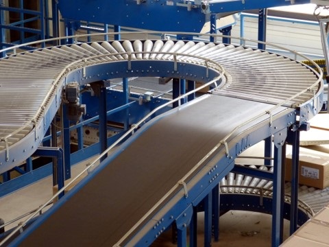
15-kg boxes are being transported around a curve via a conveyor belt, as shown below. Assuming the curve has a radius of 3 meters and the boxes are traveling at a constant speed of 1 meter per second, what is the minimum coefficient of friction needed to ensure the boxes don’t slip as they travel around the curve?

Figure \(\PageIndex{4}\): problem diagram for Example \(\PageIndex{3}\); a level section of conveyor belt in a semicircular shape.

Solution

Video \(\PageIndex{4}\): Worked solution to example problem \(\PageIndex{3}\), provided by Dr. Majid Chatsaz. YouTube source: https://youtu.be/4z73Pc3s_TE.