8.4: Equations of Motion in Polar Coordinates

Last updated
Save as PDF

Page ID: 54139

\( \newcommand{\vecs}[1]{\overset { \scriptstyle \rightharpoonup} {\mathbf{#1}} } \) \( \newcommand{\vecd}[1]{\overset{-\!-\!\rightharpoonup}{\vphantom{a}\smash {#1}}} \)\(\newcommand{\id}{\mathrm{id}}\) \( \newcommand{\Span}{\mathrm{span}}\) \( \newcommand{\kernel}{\mathrm{null}\,}\) \( \newcommand{\range}{\mathrm{range}\,}\) \( \newcommand{\RealPart}{\mathrm{Re}}\) \( \newcommand{\ImaginaryPart}{\mathrm{Im}}\) \( \newcommand{\Argument}{\mathrm{Arg}}\) \( \newcommand{\norm}[1]{\| #1 \|}\) \( \newcommand{\inner}[2]{\langle #1, #2 \rangle}\) \( \newcommand{\Span}{\mathrm{span}}\) \(\newcommand{\id}{\mathrm{id}}\) \( \newcommand{\Span}{\mathrm{span}}\) \( \newcommand{\kernel}{\mathrm{null}\,}\) \( \newcommand{\range}{\mathrm{range}\,}\) \( \newcommand{\RealPart}{\mathrm{Re}}\) \( \newcommand{\ImaginaryPart}{\mathrm{Im}}\) \( \newcommand{\Argument}{\mathrm{Arg}}\) \( \newcommand{\norm}[1]{\| #1 \|}\) \( \newcommand{\inner}[2]{\langle #1, #2 \rangle}\) \( \newcommand{\Span}{\mathrm{span}}\)\(\newcommand{\AA}{\unicode[.8,0]{x212B}}\)

To finish our discussion of the equations of motion in two dimensions, we will examine Newton's Second law as it is applied to the polar coordinate system. In its basic form, Newton's Second Law states that the sum of the forces on a body will be equal to mass of that body times the rate of acceleration. For bodies in motion, we can write this relationship out as the equation of motion.

\[ \sum \vec{F} = m * \vec{a} \nonumber \]

Just as we did with with rectangular and normal-tangential coordinates, we will break this single vector equation into two separate scalar equations. This involves identifying the \(r\) and \(\theta\) directions and then using sines and cosines to break the given forces and accelerations down into components in those directions.

The first quadrant of a Cartesian coordinate plane is depicted with a radar station at the origin, and a missile being tracked at a distance of r from the origin and an angle of Theta degrees above the x-axis. The missile is currently accelerating directly upwards in the y direction. Its net acceleration is split into acceleration in the r-direction, continuing in the direction of the r vector, and acceleration in the theta-direction, 90 degrees counterclockwise from the r-direction. The theta axis is at an angle of Theta degrees to the left of the net acceleration vector. Acceleration_theta = magnitude of net acceleration times sin(90° - Theta), and acceleration_r = magnitude of net acceleration times cos (90° - Theta). — Figure \(\PageIndex{1}\): When working in the polar coordinate system, any given forces or accelerations can be broken down using sines and cosines as long as the angle of the force or acceleration is known relative to the \(r\) and \(\theta\) directions.

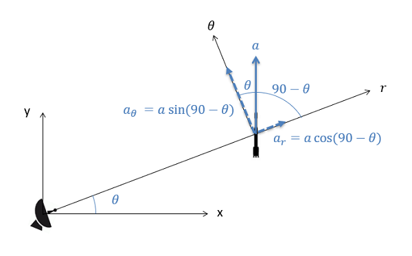
\begin{align} \sum F_r &= m * a_r \\[5pt] \sum F_{\theta} &= m * a_{\theta} \end{align}

Just as with our other coordinate systems, the equations of motion are often used in conjunction with the kinematics equations, which relate positions, velocities and accelerations as discussed in the previous chapter. In particular, we will often substitute the known values below for the \(r\) and \(\theta\) components for acceleration.

\[ a_r = \ddot{r} - r \theta^2 \]

\[ a_{\theta} = 2 \dot{r} \dot{\theta} + r \ddot{\theta} \]

Polar coordinates can be used in any kinetics problem; however, they work best with problems where there is a stationary body tracking some moving body (such as a radar dish) or there is a particle rotating around some fixed point. These equations will also come back into play when we start examining rigid body kinematics.

Video lecture covering this section, delivered by Dr. Jacob Moore. YouTube source: https://youtu.be/XiuQSSVdRKk.

Example \(\PageIndex{1}\)

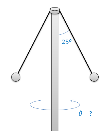
A device consists of two masses, each 0.5 kg in mass, tethered to a central shaft. The tethers are each 0.75 meters long and each tether currently makes a 25-degree angle with the central shaft. Assume the central shaft is spinning at a constant rate. What is the rate at which the shaft is spinning? If we want it to spin at exactly 100 rpm, what should the angle of the tethers be?

A vertical central shaft has two identical rope tethers dangling from the top end, one on the left side of the shaft and the other on the right side. Each tether supports an identical spherical mass and makes an angle of 25° with the shaft. The shaft is rotating in a counterclockwise direction, at the rate dot-theta. — Figure \(\PageIndex{2}\): problem diagram for Example \(\PageIndex{1}\). A spinning shaft supports two identical tethers at its top end, with each tether holding a mass and splayed out symmetrically from the shaft.

Solution: Video \(\PageIndex{2}\): Worked solution to example problem \(\PageIndex{1}\), provided by Dr. Majid Chatsaz. YouTube source: https://youtu.be/fGsoMdR1H9I.

Example \(\PageIndex{2}\)

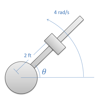
A catapult design consists of a steel weight on a frictionless rod. The rod spins at a constant rate of 4 radians per second and when \(\theta\) is 45 degrees from the horizontal, the 30-lb weight is released from its position 2 feet from the center of rotation of the shaft. What is the force the shaft exerts on the weight at the instant before and the instant after it is released? What is the acceleration of the weight along the shaft the instant after it is released?

Top-down view of a central vertical shaft that supports a horizontal rod. A weight is placed on the rod, a distance of 2 feet from the center of rotation of the vertical shaft. The rod is spinning counterclockwise at a rate of 4 rad/s, making an angle of theta with the horizontal line extending to the right of the central shaft. The current theta value is 45 degrees above that horizontal line. — Figure \(\PageIndex{3}\): problem diagram for Example \(\PageIndex{2}\). A central vertical shaft that rotates supports a horizontal rod bearing a releasable weight.

Solution: Video \(\PageIndex{3}\): Worked solution to example problem \(\PageIndex{2}\), provided by Dr. Majid Chatsaz. YouTube source: https://youtu.be/bKsi80wzLUY.