
11.2: Belt- and Gear-Driven Systems
- Page ID
- 54752

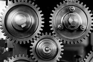
Belt-and-pulley systems, along with gear-driven systems, represent the common ways that engineers transfer rotational motion and torque from one shaft to another shaft. Belts offer flexibility in that the shafts do not need to be right next to one another, and gears are more commonly used in high-load applications.
.JPG?revision=1)
Position, Velocity, and Acceleration in Belt-Driven Systems
The diagram below shows a simple belt-driven system. Pulley A and Pulley B each have their own radius, and are connected via a belt that we will assume is not slipping relative to the pulleys. Each pulley is undergoing fixed axis rotation and will therefore follow those kinematic rules separately; however, the motion of the belt can be used to relate the motion of the two pulleys.
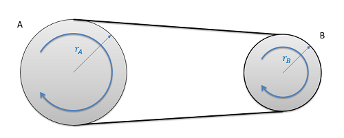
As a constraint, we can assume the speed of the pulley will be uniform throughout the whole loop at any one time. If this was not true, the belt would be bunching up in some locations and stretching out in other areas. If the belt isn't slipping, the speed of the belt will be the same as the speed of the edge of each of the two pulleys. Setting these two speeds equal to one another and working backwards to relate them to angular velocities, we wind up with the middle equation below. Taking the integral or derivative allows us to also relate angular displacements or angular accelerations with similar equations.
\begin{align} \text{Angular Displacements:} \quad &\, r_A (\Delta \theta_A) = r_B (\Delta \theta_B) \\[5pt] \text{Angular Velocities:} \quad &\, r_A \omega_A = r_B \omega_B \\[5pt] \text{Angular Accelerations:} \quad &\, r_A \alpha_A = r_B \alpha_B \end{align}
If we have a more complex series of belts and pulleys, we will analyze the system one step at at time. This will include pulleys connected via belts as we had above, as well as pulleys connected via a shaft as shown with pulleys B and C in the diagram below.
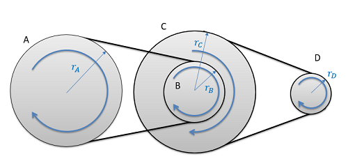
With pulleys on the same shaft, the angular displacements, the angular velocities, and the angular accelerations will all be the same.
\[ \Delta \theta_B = \Delta \theta_C \ ; \quad \omega_B = \omega_B \ ; \quad \alpha_B = \alpha_C \]
If we know the angular displacement, angular velocity, or angular acceleration of pulley A, we could find the angular displacement, angular velocity, or angular acceleration of pulley D by moving one interaction at a time (finding the motion of pulley B, then C, then D).
Position, Velocity, and Acceleration in Gear Systems:
The diagram below shows a simple gear system. Gear A and Gear B each have their own radius, and are interacting at their point of contact. Each gear is undergoing fixed-axis rotation and will therefore follow those kinematic rules separately; however, the motion of the teeth at the point of contact can be used to relate the motion of one gear to the next.
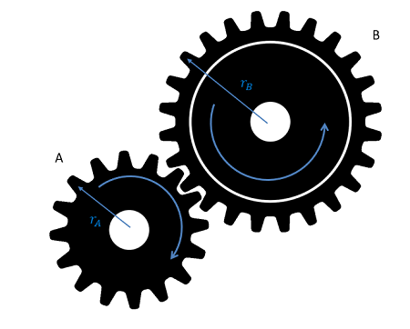
As a constraint, we can assume that the speed of the teeth at the point of contact will be the same. If this were not true, the teeth of one gear would be passing through the teeth of the other gear. Setting these these two speeds equal to one another and working backwards to relate the angular velocities, we find the second equation below. Taking the integral or derivative allows us to also relate the angular displacements or angular accelerations with similar equations.
\begin{align} \text{Angular Displacements:} \quad &\, r_A (\Delta \theta_A) = - r_B (\Delta \theta_B) \\[5pt] \text{Angular Velocities:} \quad &\, r_A \omega_A = -r_B \omega_B \\[5pt] \text{Angular Accelerations:} \quad &\, r_A \alpha_A = - r_B \alpha_B \end{align}
You will notice that the equations above match the equations we had for belt-driven systems, except for the minus sign on the right side of each equation. This is because meshed gears rotate in opposite directions (if one gear rotates clockwise, the other will rotate counterclockwise), while pulleys in belt-driven systems always rotate in the same direction.
Also similar to belt driven systems, we can have compound gear trains with three or more gears similar to the figure below. In these scenarios, we will also likely have gears that are connected via a shaft like the blue and yellow gears shown below. In such situations, the gears on the same shaft will have matching angular displacements, angular velocities, and angular accelerations. As with belt driven systems, you simply need to take the gear train one step at a time, applying the right set of equations to match each step in the interaction.
A concept that is commonly used in gear trains that is not commonly used in belt driven systems is the concept of the gear ratio. For any gear train, the gear ratio is defined as the angular speed of the input divided by the angular speed of the output. Based on the equations above, we can also prove that the ratio of angular displacements or angular accelerations will similarly be equal to the gear ratio. However, the gear ratio is always defined as a positive number, so you will still need to use intuition to determine the direction of output.
\[ \text{Gear Ratio} = \frac{\omega_{input}}{\omega_{output}} = \frac{\Delta \theta_{input}}{\Delta \theta_{output}} = \frac{\alpha_{input}}{\alpha_{output}} \]
In a simple two-gear system, the gear ratio will be equal to the radius of the output gear divided by the radius of the input gear, or the number of teeth on the output gear divided by the number of teeth on the input gear (since the number of teeth will be directly proportional to the radius). In compound gear trains this simple calculation given below will not work, but if you are given the gear ratio for a compound gear train, you can still apply the equations above.
\[ \text{Gear Ratio} = \frac{\omega_{input}}{\omega_{output}} = \frac{r_{output}}{r_{input}} = \frac{N_{output}}{N_{input}} \]
Example \(\PageIndex{1}\)
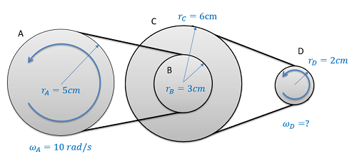
If the input pulley A as shown below is rotating at a rate of 10 rad/s, what is the speed of the output pulley at D? How many rotations does D go through in the time it takes for A to make one full rotation?
- Solution
-
Video \(\PageIndex{2}\): Worked solution to example problem \(\PageIndex{1}\), provided by Dr. Majid Chatsaz. YouTube source: https://youtu.be/IxhXp7eBx3k.
Example \(\PageIndex{2}\)
A car is moving at 40 ft/s on 18-inch-diameter wheels. What is the angular velocity of the wheels on the car? If the car is in third gear with a gear ratio of 4.89:1, what is the angular velocity of the engine in rotations per minute? (Hint: the engine is the input to the gear train and the wheels are the output of the gear train.)
- Solution
-
Video \(\PageIndex{3}\): Worked solution to example problem \(\PageIndex{2}\), provided by Dr. Majid Chatsaz. YouTube source: https://youtu.be/-2Gta-grqoI.