11.4: Relative Motion Analysis

Last updated
Save as PDF

Page ID: 54756

\( \newcommand{\vecs}[1]{\overset { \scriptstyle \rightharpoonup} {\mathbf{#1}} } \) \( \newcommand{\vecd}[1]{\overset{-\!-\!\rightharpoonup}{\vphantom{a}\smash {#1}}} \)\(\newcommand{\id}{\mathrm{id}}\) \( \newcommand{\Span}{\mathrm{span}}\) \( \newcommand{\kernel}{\mathrm{null}\,}\) \( \newcommand{\range}{\mathrm{range}\,}\) \( \newcommand{\RealPart}{\mathrm{Re}}\) \( \newcommand{\ImaginaryPart}{\mathrm{Im}}\) \( \newcommand{\Argument}{\mathrm{Arg}}\) \( \newcommand{\norm}[1]{\| #1 \|}\) \( \newcommand{\inner}[2]{\langle #1, #2 \rangle}\) \( \newcommand{\Span}{\mathrm{span}}\) \(\newcommand{\id}{\mathrm{id}}\) \( \newcommand{\Span}{\mathrm{span}}\) \( \newcommand{\kernel}{\mathrm{null}\,}\) \( \newcommand{\range}{\mathrm{range}\,}\) \( \newcommand{\RealPart}{\mathrm{Re}}\) \( \newcommand{\ImaginaryPart}{\mathrm{Im}}\) \( \newcommand{\Argument}{\mathrm{Arg}}\) \( \newcommand{\norm}[1]{\| #1 \|}\) \( \newcommand{\inner}[2]{\langle #1, #2 \rangle}\) \( \newcommand{\Span}{\mathrm{span}}\)\(\newcommand{\AA}{\unicode[.8,0]{x212B}}\)

Relative motion analysis is one method used to analyze bodies undergoing general planar motion. General planar motion is motion where bodies can both translate and rotate at the same time. Besides relative motion analysis, the alternative is absolute motion analysis. Either method can be used for any general planar motion problem, however one method may be significantly easier to apply in certain situations.

Absolute motion analysis will require calculus and is generally faster for simple problems and problems where only the velocities (and not accelerations) are required. Relative motion analysis will not require calculus, but does necessitate using multiple coordinate systems and is generally easier to use for more complex problems and problems where velocities and accelerations are being analyzed.

Utilizing Relative Motion Analysis

To start our discussion on relative motion analysis, we are going to imagine a simple robotic arm such as the one below. In this arm, we have two arm sections of fixed length, with motors causing rotations at joint A and joint B.

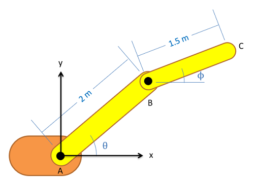
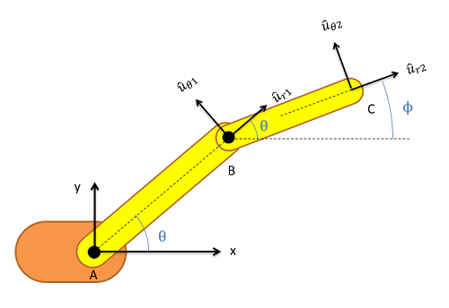
AB, a 2-meter-long robotic arm segment with its base being point A, stretches up and to the right to make an angle of theta with the positive x-axis of a standard-orientation Cartesian plane with the origin centered at point A. BC, a 1.5-meter-long robotic arm segment, connects to the free end of segment AB and stretches up and to the right, making an angle of phi with the horizontal. — Figure \(\PageIndex{1}\): This robotic arm has a fixed base at A, and two fixed length arm sections (AB and BC) that are controlled via motors at joints A and B. The end effector of the robotic arm is at C.

The first step in relative motion analysis is to break the motion down into simple steps and assign a coordinate system (with \(r\) and \(\theta\) directions) to each step in the chain of motion. We will always start at a fixed point and move step by step from there. In the case of our robotic arm, Joint A is the only point that will not be moving so we start there; then we have two cases of rotation without extension as we move from A to B, then B to C.

Since there are two steps to the motion, there will be two coordinate systems. The first coordinate system will be attached to member AB, with the \(r\) direction going from point A to point B. The \(\theta\) direction will then be ninety degrees counterclockwise from the \(r\) direction. The second coordinate system will be attached to member BC, with the \(r\) direction going from point B to point C. Again, the \(\theta\) direction is ninety degrees counterclockwise from the \(r\) direction. At this point it is usually good to identify the angles of each of the \(r\) and \(\theta\) directions with respect to ground. Below is a picture of the robotic arm with both coordinate systems drawn in.

The robotic arm from Figure 1 above, with the two new coordinate systems drawn in. The first coordinate system has its origin located at point B; its r-direction extends in the same direction as moving from A to B, and its theta-direction is 90° counterclockwise from that r-direction. The second coordinate system has its origin located at point C; its r-direction extends in the same direction as moving from B to C, and its theta-direction is 90° counterclockwise from that r-direction. — Figure \(\PageIndex{2}\): Two coordinate systems are used in the relative motion analysis of this robotic arm. The first coordinate system is attached to member AB while the second is attached to member BC. The \(r\) direction will always line up with the two endpoints of the member, while the \(\theta\) direction will always be 90° counterclockwise from the corresponding \(r\) direction.

For relative motion analysis, we can identify the velocity or acceleration of the end point of the arm (C) with respect to the ground (A) by finding the velocity acceleration of B with respect to A and adding the velocity or acceleration of C with respect to B, just as we did with particles.

\begin{align} \text{Velocity:} \quad &\, \vec{v}_{C / A} = \vec{v}_{B / A} + \vec{v}_{C / B} \\[4pt] \text{Acceleration:} \quad &\, \vec{a}_{C / A} = \vec{a}_{B / A} + \vec{a}_{B / C} \end{align}

The relative motion analysis equations above are for a two-part motion (as there are two sections to the arm in our example), but we can easily expand the above equation into three, four, or even more pieces for more complex mechanisms by adding more steps to the left side of our equation.

To use the above equations, we will need to plug in the information we know. Plugging in velocities or accelerations that are given as part of the problem for any particular points is a good place to start. If the velocity of points B or C were given, for example, we would plug that in for \(\vec{v}_{B / A}\) or \(\vec{v}_{C / A}\) respectively. Do remember that point A is our fixed ground point, so \(\vec{v}_{C / A}\) is the velocity of point C relative to the ground while \(\vec{v}_{C / B}\) is the velocity of point C with respect to point B. If any point is fixed (other than our original ground point, which will always be fixed), we can also plug in zeros for both velocity and acceleration of that point. Remember that this equation is a vector equation, so these velocities have both a magnitude and a direction.

To take into account rotation or extension of any individual pieces, we will need to look back to our kinematics equations for polar coordinator systems. Below are the equations we had for velocity and acceleration.

\begin{align} \text{Velocity:} \quad &\, v = \dot{r} \hat{u}_r + r \dot{\theta} \hat{u}_{\theta} \\[4pt] \text{Acceleration:} \quad &\, a = (\ddot{r} - r \dot{\theta}^2) \hat{u}_r + (2 \dot{r} \dot{\theta} + r \ddot{\theta}) \hat{u}_{\theta} \end{align}

In the above equations, \(r\) represents the length of the respective arm piece (the length of member AB or BC), \(\dot{r}\) represents the rate at which that length is increasing, and \(\ddot{r}\) represents the rate at which that rate is increasing. The \(\theta\) term represents current angle of the arm piece, \(\dot{\theta}\) is the angular velocity of that arm piece, and \(\ddot{\theta}\) is the angular acceleration of that arm piece. The \(u_r\) and \(u_{\theta}\) directions are the \(r\) and \(\theta\) directions that are attached to that particular section of the arm (in our earlier drawing, \(\hat{u}_{r_1}\) and \(\hat{u}_{\theta_1}\) were attached to member AB and \(\hat{u}_{r_2}\) and \(\hat{u}_{\theta_2}\) were attached to member BC).

Though it's certainly possible to have a mechanism that is rotating and extending at the same time, we will often have either just simple rotation, or just simple extension along a fixed direction. With simple rotation, the \(\dot{r}\) and \(\ddot{r}\) terms are zero, and our equations reduce down to the following.

\begin{align} \text{Velocity:} \quad &\, v = r \dot{\theta} \hat{u}_{\theta} \\[4pt] \text{Acceleration:} \quad &\, a = - r \dot{\theta}^2 \hat{u}_{r} + r \ddot{\theta} \hat{u}_{\theta} \end{align}

If we have simple extension, where the length of the piece is changing but there is no rotation, the \(\dot{\theta}\) and \(\ddot{\theta}\) terms would be zero and our original equations would reduce down to the following.

\begin{align} \text{Velocity:} \quad &\, v = \dot{r} \hat{u}_r \\ \text{Acceleration:} \quad &\, a = \ddot{r} \hat{u}_r \end{align}

If we use the appropriate set of equations for the type of motion in each step and plug in known quantities for angular velocities, angular accelerations, and rates or extension for each piece, we can add these pieces to our relative motion analysis equation from earlier. Again, these are vectors so be sure to indicate both the magnitudes and directions when we put them into the equation.

Once we have everything in our vector equation, we will break the vector equation into \(x\) and \(y\) components in order to solve for any unknowns. Simply find the angles or each of the \(r\) and \(\theta\) directions using your diagram and then use sines and cosines to break the individual vectors down into \(x\) and \(y\) components. Once you have everything in component form, you should be able to solve for any unknowns in your equations. As a note, it is often necessary to start with the velocity equations and solve for some unknowns there before moving on to the acceleration equations.

Alternate Notation for Rigid Body Relative Motion

In some cases, we want to analyze multiple points on the same or several rigid bodies. Another notation used for this is:

\begin{align} \text{Position:} \quad &\, \vec{r}_B = \vec{r}_A + \vec{r}_{B / A} \\[5pt] \text{Velocity:} \quad &\, \vec{v}_B = \vec{v}_A + \vec{v}_{B / A} = \vec{v}_A + \vec{\omega} \times \vec{r}_{B / A} \\[5pt] \text{Acceleration:} \quad &\, \vec{a}_B = \vec{a}_A + \vec{a}_{B / A} = \vec{a}_A + \vec{\alpha} \times \vec{r}_{B / A} + \vec{\omega} \times (\vec{\omega} \times \vec{r}_{B / A}) \end{align}In this notation, A and B are two points on the same rigid body. When we use only one subscript, that indicates the position/velocity/acceleration of that point with respect to the fixed coordinate system. Because the body is rigid, the two points will not change the distance between them, but the position vector between them can change orientation (which is where the relative velocity between the two points comes from). \(\vec{\omega}\) is the angular velocity of that rigid body (analogous to \(\dot{\theta}\)), and \(\vec{\alpha}\) is the angular acceleration of that rigid body (analogous to \(\ddot{\theta}\)).

For planar motion, where the angular velocity vector (out of plane) is always perpendicular to the position vector (in the plane), the acceleration can be simplified to:

\[ \text{Acceleration:} \quad \, \vec{a}_B = \vec{a}_A + \vec{\alpha} \times \vec{r}_{B / A} - \omega^2 \vec{r}_{B / A} \]

Same diagram as Figure 1 above: AB, a 2-meter-long robotic arm segment with its base being point A, stretches up and to the right to make an angle of theta with the positive x-axis of a standard-orientation Cartesian plane with the origin centered at point A. BC, a 1.5-meter-long robotic arm segment, connects to the free end of segment AB and stretches up and to the right, making an angle of phi with the horizontal. — Figure \(\PageIndex{1}\), this robotic arm has a fixed base at A, and two fixed length arm sections (AB and BC) that are controlled via motors at joints A and B. The end effector of the robotic arm is at C.

If we consider the same robotic arm, we can translate our previous notation to the new rigid body notation:

\begin{align} \dot{\theta} \hat{k} &= \vec{\omega}_{AB} \\[4pt] \dot{\phi} \hat{k} &= \vec{\omega}_{BC} \\[4pt] \ddot{\theta} \hat{k} &= \vec{\alpha}_{AB} \\[4pt] \ddot{\phi} \hat{k} &= \vec{\alpha}_{BC} \end{align}

All vectors will be defined with respect to the \(x\) and \(y\) coordinates in the coordinate system shown, rather than the radial and theta directions as above.

If we want to find the velocity and acceleration of the end point, C, knowing the angular velocities and accelerations, we will find the following relationships:

\begin{align} \text{Velocity at point B:} \quad &\, \vec{v}_B = \vec{v}_A + \vec{\omega} \times \vec{r}_{B / A} \\[5pt] \text{Velocity at point C:} \quad &\, \vec{v}_C = \vec{v}_B + \vec{\omega} \times \vec{r}_{C / B} = \vec{v}_A + \vec{\omega} \times \vec{r}_{B / A} + \vec{\omega} \times \vec{r}_{C / B} \\[5pt] \text{Acceleration at point B:} \quad &\, \vec{a}_B = \vec{a}_A + \vec{\alpha} \times \vec{r}_{B / A} - \omega^2 \vec{r}_{B / A} \\[5pt] \text{Acceleration at point C:} \quad &\, \vec{a}_C = \vec{a}_B + \vec{\alpha} \times \vec{r}_{C / B} - \omega^2 \vec{r}_{C / B} = \vec{a}_A + \vec{\alpha} \times \vec{r}_{B / A} - \omega^2 \vec{r}_{B / A} + \vec{\alpha} \times \vec{r}_{C / B} - \omega^2 \vec{r}_{C / B} \end{align}

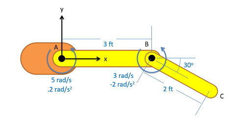
Video lecture covering this chapter, delivered by Dr. Jacob Moore. YouTube source: https://youtu.be/6qAY9iB9xi0.

Example \(\PageIndex{1}\)

The robotic arm shown below has a fixed orange base at A and fixed length members AB and BC. Motors at A and B allow for rotational motion at the joints. Based on the angular velocities and accelerations shown at each joint, determine the velocity and the acceleration of the end effector at C.

A 3-foot-long horizontal member AB is fixed to an unmoving base at its left end, point A. A motor at point A provides a counterclockwise rotation of 5 rad/s and 0.2 rad/s². A 2-foot-long member, BC, stretches down and to the right from the right endpoint of member AB, at 30° below the horizontal. A motor at point B provides a counterclockwise rotation of 3 rad/s and -2 rad/s². — Figure \(\PageIndex{4}\): problem diagram for Example \(\PageIndex{1}\). A robotic arm with two segments has motors at its joints, rotating at known velocities and accelerations.

Solution: Video \(\PageIndex{2}\): Worked solution to example problem \(\PageIndex{1}\), provided by Dr. Jacob Moore. YouTube source: https://youtu.be/fOjS1O2-3LQ.

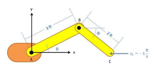
Example \(\PageIndex{2}\)

The robotic arm from the previous problem is in the configuration shown below. Assume that \(\theta\) is currently 30 degrees and that point C currently lies along the \(x\) axis. If we want the end effector at C to travel 1 ft/s in the negative \(x\)-direction, what should the angular velocities be at joints A and B?

The 3-foot-long member AB has its left endpoint, A, attached to a fixed base and stretches up and to the right, making an angle of theta above the horizontal. A standard-orientation Cartesian plane is centered at point A. The 2-foot-long member BC stretches down and to the right from the free end of AB, at an angle of phi below the horizontal. The end effector at point C, the free end of member BC, is moving horizontally leftwards at 1 ft/s (in the negative x-direction). — Figure \(\PageIndex{5}\): problem diagram for Example \(\PageIndex{2}\). A two-segmented robotic arm has an effector on its free end moving at a known speed, as a result of the rotation of the motors at the two joints.

Solution: Video \(\PageIndex{3}\): Worked solution to example problem \(\PageIndex{2}\), provided by Dr. Jacob Moore. YouTube source: https://youtu.be/esp_gz8VKRs.

Example \(\PageIndex{3}\)

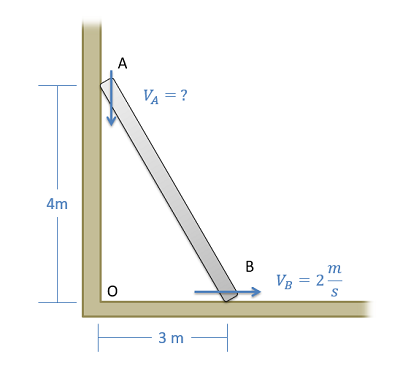
A ladder is propped up against a wall as shown below. If the base of the ladder is sliding out at a speed of 2 m/s, what is the speed of the top of the ladder?

Side view of a wall and a ladder propped against the right side of that wall. The ladder end on the wall, A, is 4 feet above the floor. The ladder end on the floor, B, is 3 feet to the right of the wall and is sliding towards the right at 2 m/s. The point of intersection between the wall and the floor is labeled as point O. — Figure \(\PageIndex{6}\): problem diagram for Example \(\PageIndex{3}\). A ladder propped against a wall is falling, as its foot slides away from the wall.

Solution: Video \(\PageIndex{4}\): Worked solution to example problem \(\PageIndex{3}\), provided by Dr. Jacob Moore. YouTube source: https://youtu.be/SzAq3HD7qJY.

Example \(\PageIndex{4}\)

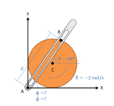
The crank-rocker mechanism as shown below consists of a crank with a radius of 0.5 meters rotating about its fixed center at C, at a constant rate of 2 rad/s clockwise. Rocker AB is fixed at its base at A and connects to point B along the edge of the crank. The pin at point B can slide along a frictionless slot in AB. In its current state, what is the angular velocity of rocker AB?

A standard-orientation first quadrant of the Cartesian plane, with the origin centered at point A. The side view of a crank is represented by a circle that is centered at point C in the first quadrant and tangent to both the x- and y-axes. The circle is rotating clockwise at 2 rad/s. A long bar with a slot cut through it has one end fixed at point A, and the pin at point B on the outer edge of the circle passes through this slot. The distance between points A and B is labeled as d. At the current position of B, the line AB makes an angle of phi with the x-axis and the line BC makes an angle of theta = 60° above the horizontal. — Figure \(\PageIndex{7}\): problem diagram for Example \(\PageIndex{4}\). A circular side view of a rotating crank with a pin in one edge. The pin moves through a slot at one end of a rocker bar, whose other end is fixed in place.

Solution: Video \(\PageIndex{5}\): Worked solution to example problem \(\PageIndex{4}\), provided by Dr. Jacob Moore. YouTube source: https://youtu.be/Exys74nj02I.