11.5: Rotating Frame Analysis

Rotating frame analysis is a specialized part of relative motion analysis. It is typically performed in Cartesian (\(x\)-\(y\)) coordinates for rigid bodies. In the previous section, rotating frames in polar coordinates were used to solve problems with formulae similar to those in particle kinematics. We will adopt a slightly different notation that is specialized to rigid bodies. These formulae are the most general planar kinematics formulae - that is, they can always be used, and will provide the correct answer. However, they are unnecessarily complicated for many types of motion, such as pure rotation.

Rotating frame analysis is really important for cases where objects are not pinned to each other. When do you use rotating frames? When one object is sliding against another object, or two objects are not even in contact, but you want to know something about the motion relationship between them and/or are given information about the motion relationship between them.

Reference Frames:

In most of the preceding material, you have worked with the fixed reference frame \(O_{xyz}\), and a translating (but not rotating) reference frame attached to the rigid body at a point \(A\), frame \(A_{xyz}\).

Figure \(\PageIndex{1}\): A rigid body with a translating (not rotating) reference frame \(x'y'z'\) attached at point \(A\), relative to the fixed frame \(xyz\) at \(O\).

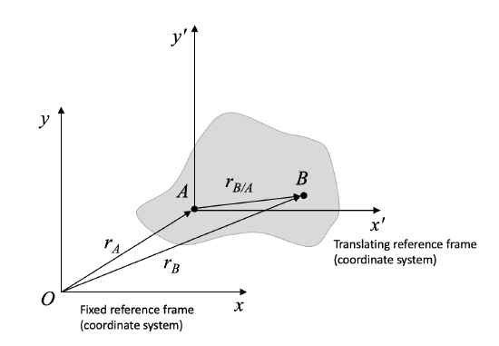
This has given us relative motion equations:

\begin{align} \text{Position:} \quad &\, \vec{r}_{B / O} = \vec{r}_{A / O} + \vec{r}_{B / A} \\ \text{Velocity:} \quad &\, \vec{v}_{B / O} = \vec{v}_{A / O} + \vec{v}_{B / A} = \vec{v}_{A / O} + \vec{\omega} \times \vec{r}_{B / A} \\ \text{Acceleration:} \quad &\, \vec{a}_{B / O} = \vec{a}_{A / O} + \vec{a}_{B / A} = \vec{a}_{A / O} + \vec{\alpha} \times \vec{r}_{B / A} - \omega^2 \vec{r}_{B / A} \end{align}

Note that the notation \(r_{B / O}\), where \(O\) is the fixed frame, can also be written as \(r_B\). Both indicate an absolute position (or velocity or acceleration) - that is, a value with respect to the fixed frame \(O\).

Rotating Frames:

Now, we will consider a reference frame that is attached to a point on the rigid body and both rotating and translating with the rigid body. We will introduce some extra terms to account for the rotation of the frame.

Consider a rigid body with frame \(x'y'z'\) at point \(A\). \(x'y'z'\) moves and rotates with the body. A bug, \(B\), is crawling along the body.

Figure \(\PageIndex{2}\): A rigid body with a translating AND rotating reference frame, \(x'y'z'\), attached at point \(A\). A bug, \(B\), is crawling along the rigid body, with a velocity relative to the rotating frame. The bug is currently above a sticker, \(C\), that is rigidly fixed to the rigid body.

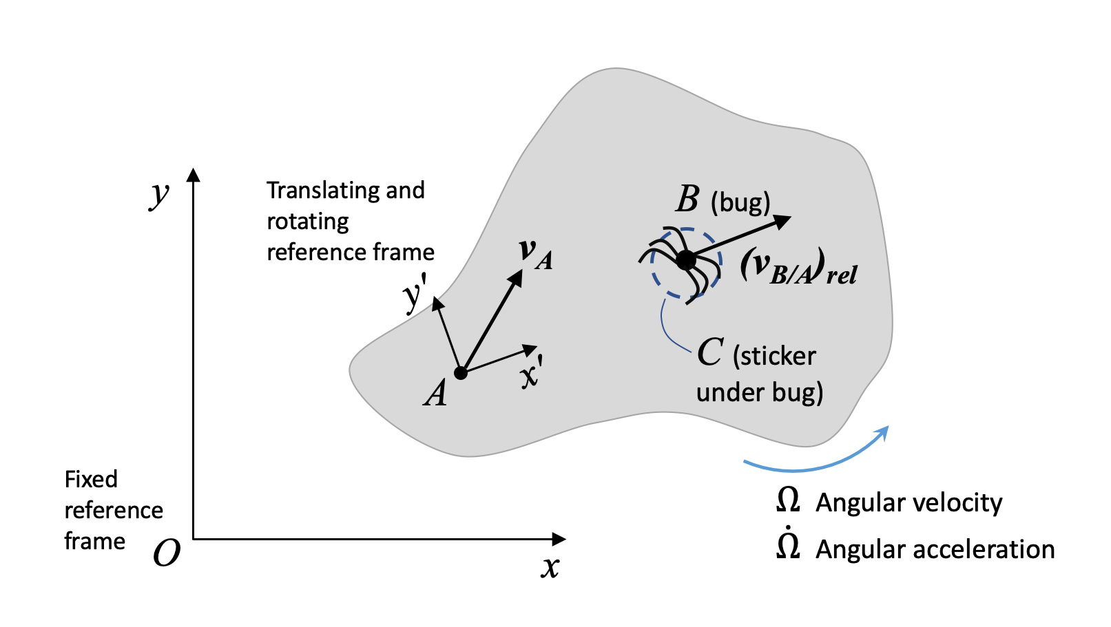
For an observer sitting at \(A\), the bug appears to be crawling away in a straight line. But for an observer sitting at \(O\), the bug does not look like it is moving in a straight line, because the body it is crawling on is also moving (translating and rotating). We would like to describe the motion of the bug as seen by an observer at \(O\). To remind ourselves that we are dealing with a rotating frame attached to one body, we use capital omega \(\Omega\)) to denote the angular velocity of the object that the rotating frame is attached to, and \(\dot{\Omega}\) for the angular acceleration of the object with the rotating frame attached. Finally, we use brackets and the subscript \(rel\) to denote values of velocity or acceleration expressed with respect to the rotating frame.

Recall that vectors have both magnitude and direction. We can express a vector in components with respect to the \(\hat{i}\) and \(\hat{j}\) unit vectors:

\[ \vec{r}_{B / O} = r_{B/O, x} \hat{i} + r_{B/O, y} \hat{j} \]

Normally, when we take a time derivative of such an expression, the length of the vector (i.e. the \(r_{B/O, x}\) and \(r_{B/O, y}\) terms) change, but the unit vectors do not. In the case of the rotating frame, the unit vectors change. Now, they don't change in length - they remain unit vectors. But they are attached to a rotating body, which means they also rotate. That is, their directions change, and we have to account for that when deriving velocity and acceleration expressions.

Figure \(\PageIndex{3}\): When the reference frame rotates with the rotating rigid body, the unit vectors change with time.

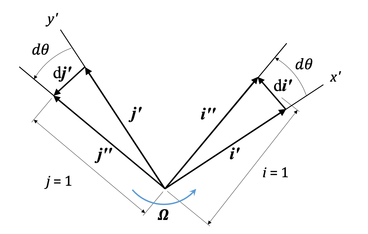
You can see we get small vectors \(d \hat{i'}\) and \(d \hat{j'}\) that describe the change in direction of the unit vectors, and the magnitude of that change is directly related to \(\Omega\), the angular velocity of the rigid body and the rotating frame.

\[ \frac{d \hat{i'}}{dt} = \Omega \hat{k} \times \hat{i'} = \Omega \hat{j'} \]

\[ \frac{d \hat{j'}}{dt} = \Omega \hat{k} \times \hat{j'} = -\Omega \hat{i'} \]

When we differentiate the relative position of the bug, \(B\), with respect to the rotating frame, \(A\), we have:

\[\frac{d \vec{r}_{B/A}}{dt} = \left( \dot{r}_{B/A, \ x'} \ \hat{i'} + \dot{r}_{B/A, \ y'} \ \hat{j'} \right) + \vec{\Omega} \times \left( r_{B/A, \ x'} \ \hat{i'} + r_{B/A, \ y'} \hat{j'} \ \right) \]

\begin{align} \text{New term:} \quad &\, \left( \dot{r}_{B/A, \ x'} \ \hat{i'} + \dot{r}_{B/A, \ y'} \ \hat{j'} \right) = \left( \vec{v}_{B/A} \right) _{rel} \\ \text{Same as before:} \quad &\, \vec{\Omega} \times \left( r_{B/A, \ x'} \ \hat{i'} + r_{B/A, \ y'} \ \hat{j'} \right) = \vec{\Omega} \times \vec{r}_{B/A} \end{align}

The new term above describes the motion of the bug due to the rotation of the rigid body (and the \(x'y'z'\) frame), while the familiar term above describes the motion of the bug as seen by an observer fixed to \(x'y'z'\). Our final expression for the velocity of the bug with respect to the fixed frame is:

\[ \vec{v}_{B/O} = \vec{v}_{A/O} + \vec{\Omega} \times \vec{r}_{B/A} + ( \vec{v}_{B/A} )_{rel} \]

This final expression has the new term, \( (\vec{v}_{B/A})_{rel} \), which describes the motion of the bug as viewed from the rotating frame. You can note that if the bug is not moving, \( (\vec{v}_{B/A})_{rel} = 0\), and we get the familiar expression from the translating, non-rotating frames. Thus, this expression is the most general relative velocity expression.

We can similarly derive an acceleration equation by differentiating the above velocity equation. The final expression is:

\[ \vec{a}_{B/O} = \vec{a}_{A/O} + \dot{\vec{\Omega}} \times \vec{r}_{B/A} + \vec{\Omega} \times ( \vec{\Omega} \times \vec{r}_{B/A} ) + 2 \vec{\Omega} \times (\vec{v}_{B/A})_{rel} + (\vec{a}_{B/A})_{rel} \]

Table \(\PageIndex{1}\): Physical correspondences of Equation \(\PageIndex{11}\) components

Motion of rotating frame attached to rigid body:	\( \vec{a}_{A/O} + \dot{\vec{\Omega}} \times \vec{r}_{B/A} + \vec{\Omega} \times ( \vec{\Omega} \times \vec{r}_{B/A} ) \)
Coriolis acceleration - interaction of object motion with respect to rotating frame and motion of rotating frame:	\( 2 \vec{\Omega} \times (\vec{v}_{B/A})_{rel} \)
Motion of object with respect to rotating frame:	\( ( \vec{a}_{B/A} )_{rel} \)

Note that, for planar (2D) motion:

\[ \vec{\Omega} \times ( \vec{\Omega} \times \vec{r}_{B/A} ) = - \Omega^2 \vec{r}_{B/A} \]

Again, if the bug is sitting still, both \(rel\) terms become zero (it is not moving with respect to the rigid body), and we are left with the same relative motion expression used with translating frames. So, Equation \(\PageIndex{11}\) is the most general form of the relative acceleration equation and can always be used.

When tackling these problems, there are several important things to remember:

1. You need to pick the correct body to attach the rotating frame to. The correct body will have another body sliding against it. If the object of interest is pinned to the body you chose, it might not be correct.
2. It is often helpful to align your rotating frame such that you end up with a simplified "\(rel\)" term or terms. For example, line up the \(x'\) axis with the direction of movement of the bug, so that \( (\vec{v}_{B/A})_{rel} \) is in the \(x'\)-direction.
3. The components of all terms of any one equation must be computed along the same \(\hat{i}\) and \(\hat{j}\) directions. If the frames are not aligned, you must pick ONE FRAME and express all terms along that the directions of the ONE FRAME. (You may be able to switch between frames in different equations, but make sure you are careful with notation!)
4. When you are given information in a problem, pay careful attention to what frame is being referred to.
5. Make sure you include all the terms in the acceleration equation! It's easy to miss one. You should have five terms.

These are some of the most complex problems in planar kinematics, so take your time!

Exercise \(\PageIndex{1}\)

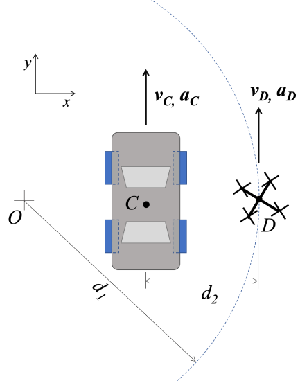
A camera drone, \(D\), flies over a car race in a curved trajectory (center \(O\)) with a constant ground-speed velocity of \(v_D = 9 \ m/s\). At the moment shown, car \(C\) is traveling with velocity of \(v_c = 12 \ m/s\) and an acceleration of \(a_c = 2 \ m/s^2\) as shown. Assume \(d_1 = 7.5 \ m, \ d_2\) = \ 3 m\).

• Find the velocity of the car as observed by the camera on drone D at this instant.
• Find the acceleration of the car as observed by the camera on drone D at this instant.

Figure \(\PageIndex{4}\): problem diagram for Example \(\PageIndex{1}\). A drone tracing a circular path around point \(O\) is currently straight to the right of a car, with the velocity and acceleration vectors of the two vehicles pointing in the same direction.

Solution

Video \(\PageIndex{1}\): Worked solution to example problem \(\PageIndex{1}\), provided by Dr. Jacob Moore. YouTube source: https://youtu.be/nqs7bLBVm3g.

Example \(\PageIndex{2}\)

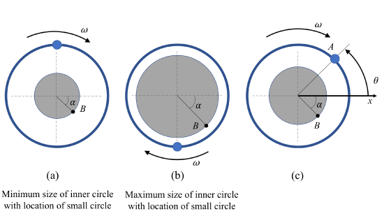
A breathing exercise video graphic (somewhat similar to this one) shows a small circle moving in a constrained circular path (constant radius 80 cm) at a constant angular velocity of 0.4 rad/s around an expanding and contracting inner circle. The inner circle expands and contracts sinusoidally, from a minimum radius of 30 cm to a maximum radius of 60 cm. The distance from the center of the inner circle to a point on the edge of the inner circle can be described by the equation \(r = 0.45 - 0.15 \sin (\theta)\), where \(r\) is in meters and \(\theta\) is the position of the small circle (zero at the \(x\)-axis).

Find the velocity and acceleration of point B on the edge of the inner circle as viewed by an observer on the small circle at point \(A\) (see part C of the figure below). \(\theta = 45\)°, \(\alpha = 45\)°

Figure \(\PageIndex{5}\): problem diagram for Example \(\PageIndex{2}\). A large circular outline rotates at a constant rate, changing the location of a small circle attached to it, while an inner circle concentric with the outline expands and contracts in radius.

Solution

Video \(\PageIndex{2}\): Worked solution to example problem \(\PageIndex{2}\), provided by Dr. Jacob Moore. YouTube source: https://youtu.be/mL0PVJNnOBE.