
13.1: Conservation of Energy for Rigid Bodies
- Page ID
- 54803

The concepts of Work and Energy provide the basis for solving a variety of kinetics problems. Generally, this method is called the Energy Method or the Conservation of Energy, and it can be boiled down to the idea that the work done to a body will be equal to the change in energy of that body. Dividing energy into kinetic and potential energy pieces as we often do in dynamics problems, we arrive at the following base equation for the conservation of energy.
\[ W = \Delta KE + \Delta PE \]
It is important to notice that unlike Newton's Second Law, the above equation is not a vector equation. It does not need to be broken down into components which can simplify the process. However, we only have a single equation and therefore can only solve for a single unknown, which can limit this method.
Work in Rigid Body Problems:
For work done to a rigid body, we must consider any force applied over a distance as we did for particles, as well as any moment exerted over some angle of rotation. If these are constant forces and constant moments, we simply multiple the force times the distance and the moment times the angle of rotation to find the overall work done in the problem. As with particles, these are the components of forces in the direction of travel, with forces opposing the motion counting as negative work. Similarly, these are moments in the direction of rotation, with moments opposing the rotation counting as negative work. Both types of work are additive, with all work being lumped together for analysis.
\[ W = F * d + M * \Delta \theta \]
In instances of non-constant forces and non-constant moments, we will need to integrate the forces and moments over the distance traveled and the angle of rotation, respectively.
\[ W = \int \limits_{x_1}^{x_2} F(x) \, dx + \int \limits_{\theta_1}^{\theta_2} M(\theta) \, d \theta \]
Energy:
In rigid bodies, as with particles, we will break energy into kinetic energy and potential energy. Kinetic energy is the the energy mass in motion, while potential energy represents the energy that is stored up due to the position or stresses in a body.
In its equation form, the kinetic energy of a rigid body is represented by one-half of the mass of the body times its velocity squared, plus one-half of the mass moment of inertia times the angular velocity squared. If we wish to determine the change in kinetic energy, we would simply take the final kinetic energy minus the initial kinetic energy.
\[ KE = \frac{1}{2} m v^2 + \frac{1}{2} I \omega^2 \]
\[ \Delta KE = \left( \frac{1}{2} m v_f^2 - \frac{1}{2} m v_i^2 \right) + \left( \frac{1}{2} I \omega_f^2 - \frac{1}{2} I \omega_i^2 \right) \]
Potential energy, unlike kinetic energy, is not really energy at all. Instead, it represents the work that a given force will potentially do between two instants in time. Potential energy can come in many forms, but the two we will discuss here are gravitational potential energy and elastic potential energy. These represent the work that the gravitational force and a spring force will do, respectively. We often use these potential energy terms in place of the work done by gravity or springs respectively. When including these potential energy terms, it's important to not also include the work done by gravity or spring forces.
The change in gravitational potential energy for any system is represented by the mass of the body, times the value \(g\) (9.81 m/s2 or 32.2 ft/s2 on the earth's surface), times the vertical change in height between the start position and the end position. In equation form, this is as follows. \[ \Delta PE = m * g * \Delta h \]
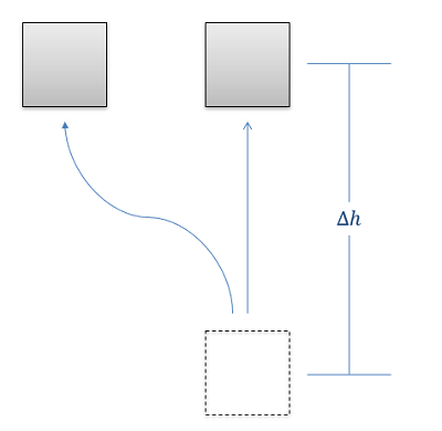
Unlike work and kinetic energy, there is no rotational version of gravitational potential energy, so this is exactly the same as we had for particles.
To determine the change in elastic potential energy, we will have to identify any linear springs (as we had for particles), as well as any torsional springs and the spring constants for each of these springs.
To find the change in elastic potential energy, we will need to know the stiffness of any spring in the problem (represented by \(k\), in units of force per distance for linear springs or moment per angle of twist for torsional springs) as well as the distance or angle the spring has been stretched above or below its natural resting position. This difference from resting position is represented by distance \(x\) for linear springs, or angle \(\theta\) for torsional springs. Once we have those values, the elastic potential energy can be calculated by multiplying one-half of the stiffness by the distance \(x\) squared or the angle \(\theta\) squared. To find the change in elastic potential energy, we simply take the final elastic potential energy minus the initial elastic potential energy.
\[ \Delta PE_{linear \ spring} = \frac{1}{2} k \ x_f^2 - \frac{1}{2} k \ x_i^2 \]
\[ \Delta PE_{torsional \ spring} = \frac{1}{2} k \ \theta_f^2 - \frac{1}{2} k \ \theta_i^2 \]
Going back to our original conservation of energy equation, we simply plug the appropriate terms on each side (work on the left and energies on the right) and balance the two sides to solve for any unknowns. Terms that do not exist or do not change (such as elastic potential energy in a problem with no springs, or \(\Delta KE\) in a problem where there is no change in the speed of the body) can be set to zero. Again, there is only one equation, so we can only solve for a single unknown unless we supplement the conservation of energy equation with other relationship equations.
Example \(\PageIndex{1}\)
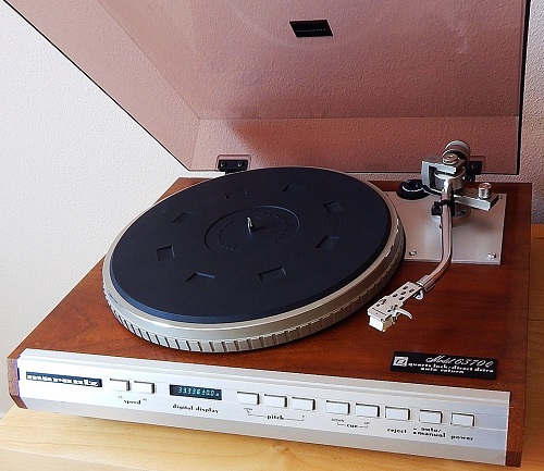
The turntable on a record player consists of a disk 12 inches in diameter with a weight of 5 lbs. The motor accelerates the turntable from rest to its operating speed of 33.33 rpm in one rotation. What is the work done by the motor? What is the average torque the motor exerted?
- Solution
-
Video \(\PageIndex{2}\): Worked solution to example problem \(\PageIndex{1}\), provided by Dr. Majid Chatsaz. YouTube source: https://youtu.be/UPHgU-o80Q0.
Example \(\PageIndex{2}\)
A system as shown below is used to passively slow the lowering of a gate. The gate can be approximated as a flat plate on its edge with a mass of 25 kilograms and a height of 2 meters. Assume the spring is unstretched as shown in the diagram.
- What would the angular velocity of the gate be without the spring?
- If we want to reduce the angular velocity at the bottom to 25% of its original value, what should the spring constant be?
- Solution
-
Video \(\PageIndex{3}\): Worked solution to example problem \(\PageIndex{2}\), provided by Dr. Majid Chatsaz. YouTube source: https://youtu.be/HCAC0tNR18w.
Example \(\PageIndex{3}\)
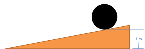
A 5-kilogram spherical ball with a radius of 0.05 meters is placed on a ramp as shown below. If the ball rolls without slipping, what is the velocity of the ball at the bottom of the ramp?
- Solution
-
Video \(\PageIndex{4}\): Worked solution to example problem \(\PageIndex{3}\), provided by Dr. Majid Chatsaz. YouTube source: https://youtu.be/p2pvQ0kCWIU.
Example \(\PageIndex{4}\)
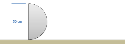
A 16-kilogram half-cylinder is placed on a hard, flat surface as shown below and released from rest. What will the maximum angular velocity be as it rocks back and forth?
- Solution
-
Video \(\PageIndex{5}\): Worked solution to example problem \(\PageIndex{4}\), provided by Dr. Majid Chatsaz. YouTube source: https://youtu.be/HpRtDQjoEBA.
Example \(\PageIndex{5}\)
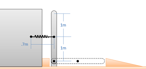
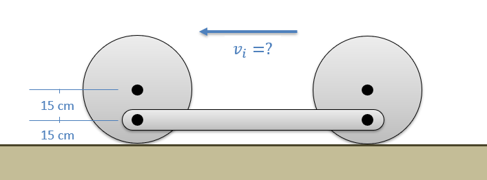
A mechanism consists of two 3-kilogram wheels connected to a 2-kilogram bar as shown below. Based on the dimensions in the diagram, what is the minimum required initial velocity for the wheels to ensure the mechanism makes it all the way through one rotation without rocking backwards?
- Solution
-
Video \(\PageIndex{6}\): Worked solution to example problem \(\PageIndex{5}\), provided by Dr. Majid Chatsaz. YouTube source: https://youtu.be/8cjQ1S6yOTc.