15.1: Undamped Free Vibrations

Last updated
Save as PDF

Page ID: 50618

\( \newcommand{\vecs}[1]{\overset { \scriptstyle \rightharpoonup} {\mathbf{#1}} } \) \( \newcommand{\vecd}[1]{\overset{-\!-\!\rightharpoonup}{\vphantom{a}\smash {#1}}} \)\(\newcommand{\id}{\mathrm{id}}\) \( \newcommand{\Span}{\mathrm{span}}\) \( \newcommand{\kernel}{\mathrm{null}\,}\) \( \newcommand{\range}{\mathrm{range}\,}\) \( \newcommand{\RealPart}{\mathrm{Re}}\) \( \newcommand{\ImaginaryPart}{\mathrm{Im}}\) \( \newcommand{\Argument}{\mathrm{Arg}}\) \( \newcommand{\norm}[1]{\| #1 \|}\) \( \newcommand{\inner}[2]{\langle #1, #2 \rangle}\) \( \newcommand{\Span}{\mathrm{span}}\) \(\newcommand{\id}{\mathrm{id}}\) \( \newcommand{\Span}{\mathrm{span}}\) \( \newcommand{\kernel}{\mathrm{null}\,}\) \( \newcommand{\range}{\mathrm{range}\,}\) \( \newcommand{\RealPart}{\mathrm{Re}}\) \( \newcommand{\ImaginaryPart}{\mathrm{Im}}\) \( \newcommand{\Argument}{\mathrm{Arg}}\) \( \newcommand{\norm}[1]{\| #1 \|}\) \( \newcommand{\inner}[2]{\langle #1, #2 \rangle}\) \( \newcommand{\Span}{\mathrm{span}}\)\(\newcommand{\AA}{\unicode[.8,0]{x212B}}\)

Vibrations occur in systems that attempt to return to their resting or equilibrium state when perturbed, or pushed away from their equilibrium state. The simplest vibrations to analyze are undamped, free vibrations with one degree of freedom.

"Undamped" means that there are no energy losses with movement (whether the losses are intentional, from adding dampers, or unintentional, through drag or friction). An undamped system will vibrate forever without any additional applied forces. A simple pendulum has very low damping, and will swing for a long time before stopping. "Damped" means that there are resistive forces and energy losses with movement that cause the system to stop moving eventually.

"Free" means that, after the initial perturbation, the only forces acting on the system are internal to the system (springs, dampers) and/or gravity. A tuning fork continues to vibrate after the one initial perturbation of being struck. In contrast, "forced" means there is an external, typically periodic, force acting on the system. A jackhammer vibrates due to having a supply of compressed air continually forcing the bit up and down, and it stops vibrating very quickly without that external periodic forcing.

"One degree of freedom" means that we will only consider systems with one mass vibrating along one direction (e.g. use variable \(x\)) or about one axis (e.g. use variable \(\theta\)). Systems having more than one mass or vibrating along or about two or more axes have more than one degree of freedom.

We can derive the equation of the system by setting up a free body diagram. Consider a mass sitting on a frictionless surface, attached to a wall via a spring.

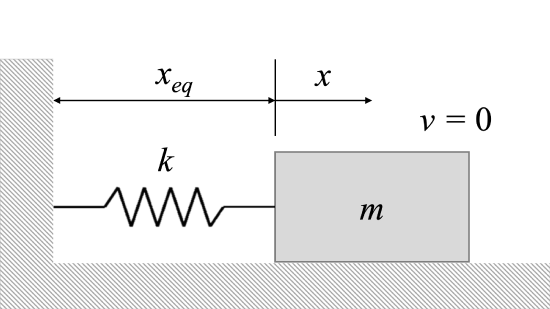
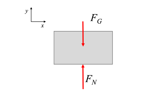
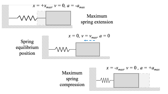
A block of mass m is at rest on a flat surface. A spring of spring constant k is attached to the left side of the block, and the left end of that spring is attached to a wall. The current length of the spring, which is at equilibrium, is x_eq, and the direction of increasing x is towards the right. — Figure \(\PageIndex{1}\): This is a system consisting of a mass attached to the wall via a spring, sitting on a frictionless surface. The system is currently in equilibrium, and the spring is not stretched or compressed.

The system above is in equilibrium. It is at rest, and will stay at rest unless some other force acts on it.

Free body diagram of the rectangular mass from Figure 1 above. It experiences a downwards gravitational force from the Earth, and an upwards normal force, of the same magnitude, from the surface it is sitting on. — Figure \(\PageIndex{2}\): Free body diagram of the system in equilibrium position. Since the spring is at its unstretched length, it does not produce a force.

To start the system vibrating, we need to perturb it. Perturbation is moving the system away from equilibrium by a small amount.

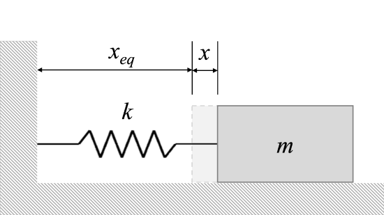
The system from Figure 1 above has the mass moved a small distance x towards the right from its equilibrium position. — Figure \(\PageIndex{3}\): Mass-spring system perturbed by an amount \(+x\) from equilibrium. This stretches the spring, causing a spring force which tends to pull the mass back toward equilibrium.

When we perturb this system, we either stretch or compress the spring. This generates a spring force, and the spring force is always in a direction that tends to pull the system back toward equilibrium.

Free body diagram of the mass from Figure 3 above. It experiences a downwards force from gravity balanced by an upwards normal force from the surface it sits on, as well as a force pointing towards the left as the stretched spring attempts to return to its equilibrium length. — Figure \(\PageIndex{4}\): Free body diagram of the mass-spring system perturbed by an amount \(+x\) from equilibrium. This stretches the spring, causing a spring force which tends to pull the mass back toward equilibrium.

The mass-spring system at three different positions, with their respective x-position, velocity, and acceleration values, with positive values pointing to the right and negative to the left. One position is maximum spring extension, where x = x_max, v = 0, and a = -a_max. The second is the spring equilibrium position, where x = 0, v = - v_max, and a = 0. The third position is maximum spring compression, where x = -x_max, v = 0, and a = a_max. — Figure \(\PageIndex{5}\): Mass-spring system vibration. After an initial perturbation, the system oscillates between two extreme positions (\(-x_{max}\) and \(x_{max}\)). The extreme positions are turnaround points where the velocity is zero, but the spring force is at a maximum (maximum stretch/compression) and therefore the acceleration is maximum. As the system passes through the equilibrium position, the spring is no longer stretched (zero force, zero acceleration), but the velocity is at its maximum (this can be determined using conservation of energy) and the inertia of the system carries the mass past the equilibrium position. In the absence of damping or the application of another force, the system will oscillate forever.

We can generate the equation of motion of the system, and determine the specifics of how it will vibrate, by analyzing this perturbed state. Recall that the spring force or moment is:

\[ \vec{F}_k = k \vec{x} \]

\[ \vec{M}_k = k \vec{\omega} \]

Note that the spring constants in the above equations have different units, depending on whether the spring is linear (Newton/meter) or torsional (Newton-meter/radian), and that \(\theta\) must be given in radians. The magnitude of the spring force depends on \(x\), the distance perturbed from the spring's unstretched length (not necessarily the equilibrium position of the system), and the same is true for the moment of a torsional spring. The spring force or moment is in the direction/orientation opposite that of the displacement. That is, if you pull the mass to the right, the spring force points to the left.

The process for finding the equation of motion of the system is as follows:

Sketch the system with a small positive perturbation (\(x\) or \(\theta\)).
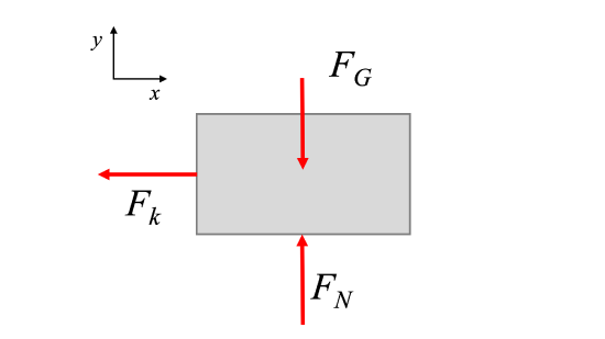
Draw the free body diagram of the perturbed system. Ensure that the spring force has a direction opposing the perturbation.
Find the one equation of motion for the system in the perturbed coordinate using Newton's Second Law. Keep the same positive direction for position, and assign positive acceleration in the same direction.
Move all terms of the equation to one side, and check that all terms are positive. If all terms are not positive, there is an error in the direction of displacement, acceleration, and/or spring force.

For the example system above, with mass \(m\) and spring constant \(k\), we derive the following:

\[ \sum F_x = m a_x = m \ddot{x} \]

\[ -F_k = m \ddot{x} \]

\[ -kx = m \ddot{x} \]

\[ m \ddot{x} + kx = 0 \]

This gives us a differential equation that describes the motion of the system. We can rewrite it in normal form:

\[ m \ddot{x} + kx = 0 \]

\[ \Rightarrow \ddot{x} + \frac{k}{m} x = 0 \]

\[ \Rightarrow \ddot{x} + \omega_n^2 x = 0 \]

The term \(\omega_n\) is called the angular natural frequency of the system, and has units of radians/second.

\[ \omega_n^2 = \frac{k}{m} \]

\[ \omega_n = \sqrt{\frac{k}{m}} \]

Assuming that the initial perturbation of the system can be described by the position and velocity of the mass at \(t=0\), then:

\[ x(0) = x_0 \]

\[ v(0) = \dot{x}(0) = v_0. \]

The solution to the differential equation, that provides the position \(x(t)\) of the system at time \(t\), is:

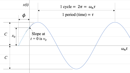
\[ x(t) = C \sin \left( \omega_n t + \phi \right), \]

\[ \text{where:} \quad \omega_n = \sqrt{\frac{k}{m}}, \,\, C = \sqrt{ \left( \frac{v_0}{\omega_n} \right)^2 + x_0^2 }, \,\, \phi = \tan ^{-1} \left( \frac{x_0 \omega_n}{v_0} \right). \]

The amplitude \(C\) describes the maximum displacement during the oscillations (i.e. \(x_{max}\)), and the phase \(\phi\) describes how the sine function is shifted in time.

Graph of a sine function on a horizontal axis of omega_n t and a vertical axis of x(t), starting at t=0. The sine graph has been shifted slightly to the left, so there is a distance of phi between the vertical axis and the closest intersection of the horizontal axis with the projected graph to the left of t=0. C is the amplitude, or the distance between the horizontal axis and the highest or lowest points of the sine function; the slope of the graph at t=0 is v_0; and there is a cycle of 2 pi units, or omega_n * tau where tau is the period, between two adjacent maxima or minima of the graph. — Figure \(\PageIndex{6}\): Displacement response of the mass spring system (solution to the differential equation).

For a system where there is torsional vibration (that is, the oscillation involves a rotation), the equations are similarly:

\[ I \ddot{\theta} + k \theta = 0 \]

\[ \Rightarrow \ddot{\theta} + \frac{k}{I} \theta = 0 \]

\[ \Rightarrow \ddot{\theta} + \omega_n^2 \theta = 0, \]

\[ \text{where} \,\, \omega_n = \sqrt{\frac{k}{I}}. \]

Assuming that the initial perturbation of the system can be described by the position and velocity of the mass at \(t=0\),

\[x(0) = x_0 \]

\[ v(0) = \dot{x}(0) = v_0. \]

The solution to the differential equation, that provides the position \(x(t)\) of the system at time \(t\), is:

\[ x(t) = C \sin (\omega_n t + \phi) \]

\[ \text{where:} \quad \omega_n = \sqrt{\frac{k}{I}}, \,\, C = \sqrt{ \left( \frac{\omega_0}{\omega_n} \right) ^2 + \theta_0^2 }, \,\, \phi = \tan ^{-1} \left( \frac{\theta_0 \omega_n}{\omega_0} \right). \]

Example \(\PageIndex{1}\)

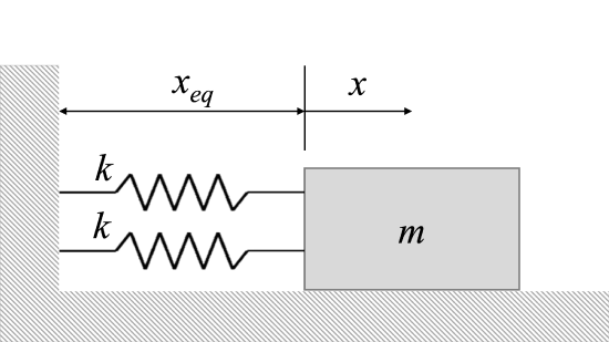
Find an expression for the angular natural frequency of the following system, and find the maximum amplitude of vibration of the system with mass \(m\) = 10 kg and spring constant \(k\) = 200 N/m when given an initial displacement of \(x_0\) = 0.1 m and an initial velocity of \(v_0\) = 0.3 m/s.

A rectangular mass m sits on a flat surface. The left edge of the mass is attached to the right ends of two identical horizontal springs, one above the other. The left end of each spring is attached to a wall. The springs are currently at their equilibrium length x_eq, and the mass is at position x = 0 with the positive x-direction being to the right. — Figure \(\PageIndex{7}\): problem diagram for Example \(\PageIndex{1}\). A rectangular mass on a flat surface has its left edge attached to two identical springs, whose other ends are attached to a wall.

Solution: Video \(\PageIndex{1}\): Worked solution to example problem \(\PageIndex{1}\). YouTube source: https://youtu.be/J1TVxxVjV_c.

Example \(\PageIndex{2}\)

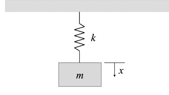
Determine the equation of motion of the system from Newton's Second Law. Assume mass \(m\) = 5 kg and spring constant \(k\) = 500 N/m. Find the initial displacement, \(x_0\), such that the mass oscillates over a total range of 4 meters. Assume the initial perturbation velocity, \(v_0\), is 10 m/s.

A vertical spring hangs from a ceiling. A mass m is attached to the free end of the spring, and the system is at rest. The positive x-direction points towards the bottom of the page, with the current position of the mass being x = 0. — Figure \(\PageIndex{8}\): problem diagram for Example \(\PageIndex{2}\). A mass hangs from a spring attached to a ceiling.

Solution: Video \(\PageIndex{2}\): Worked solution to example problem \(\PageIndex{2}\). YouTube source: https://youtu.be/TAy412iVvwE.