17.6: Mass Moments of Inertia via Integration

Last updated
Save as PDF

Page ID: 55343

\( \newcommand{\vecs}[1]{\overset { \scriptstyle \rightharpoonup} {\mathbf{#1}} } \) \( \newcommand{\vecd}[1]{\overset{-\!-\!\rightharpoonup}{\vphantom{a}\smash {#1}}} \)\(\newcommand{\id}{\mathrm{id}}\) \( \newcommand{\Span}{\mathrm{span}}\) \( \newcommand{\kernel}{\mathrm{null}\,}\) \( \newcommand{\range}{\mathrm{range}\,}\) \( \newcommand{\RealPart}{\mathrm{Re}}\) \( \newcommand{\ImaginaryPart}{\mathrm{Im}}\) \( \newcommand{\Argument}{\mathrm{Arg}}\) \( \newcommand{\norm}[1]{\| #1 \|}\) \( \newcommand{\inner}[2]{\langle #1, #2 \rangle}\) \( \newcommand{\Span}{\mathrm{span}}\) \(\newcommand{\id}{\mathrm{id}}\) \( \newcommand{\Span}{\mathrm{span}}\) \( \newcommand{\kernel}{\mathrm{null}\,}\) \( \newcommand{\range}{\mathrm{range}\,}\) \( \newcommand{\RealPart}{\mathrm{Re}}\) \( \newcommand{\ImaginaryPart}{\mathrm{Im}}\) \( \newcommand{\Argument}{\mathrm{Arg}}\) \( \newcommand{\norm}[1]{\| #1 \|}\) \( \newcommand{\inner}[2]{\langle #1, #2 \rangle}\) \( \newcommand{\Span}{\mathrm{span}}\)\(\newcommand{\AA}{\unicode[.8,0]{x212B}}\)

The mass moment of inertia represents a body's resistance to angular accelerations about an axis, just as mass represents a body's resistance to linear accelerations. This is represented in an equation with the rotational version of Newton's Second Law.

\[ F = ma \]

\[ M = I \alpha \]

Just as with area moments of inertia, the mass moment of inertia can be calculated via moment integrals or via the method of composite parts and the parallel axis theorem. This page will only discuss the integration method, as the method of composite parts is discussed on a separate page.

The Mass Moment of Inertia and Angular Accelerations

The mass moment of inertia is a moment integral, specifically the second polar mass moment integral. To see why this relates moments and angular accelerations, we start by examining a point mass on the end of a massless stick as shown below. Imagine we want to rotate the stick about the left end by applying a moment there. We want to relate the moment exerted to the angular acceleration of the stick about this point.

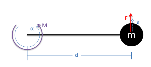
A horizontal stick of length d holds a point mass on its right end. A counterclockwise moment and angular acceleration are applied to the left end of the stick, causing the point mass to experience a force and an acceleration that point towards the top of the page. — Figure \(\PageIndex{1}\): A point mass on the end of a massless stick. We are attempting to rotate the mass about the stick's left end by exerting a moment there.

To relate the moment and the angular acceleration, we need to start with the traditional form of Newton's Second Law, stating that the force exerted on the point mass by the stick will be equal to the mass times the acceleration of the point mass (\(F = m*a\)). In this case the moment will be related to the force in that the force exerted on the mass times the length of the stick (\(d\)) is equal to the moment. We can also relate the linear acceleration of the mass to its rotational counterpart in that the linear acceleration is the angular acceleration times the length of the rod (\(d\)). If we take these two substitutions and put them into the original \(F = m*a\) equation, we can wind up with an equation that relates the moment and the angular acceleration for our scenario. A simplified version of this new relationship states that the moment will be equal to the mass times the distance squared times the angular acceleration. This mass-times-distance-squared term (relating the moment and angular acceleration) forms the basis for the mass moment of inertia.

\[ F = m * a \]

\[ M = F * d \quad\quad\quad a = d * \alpha \]

\[ M = (m * d^2) * \alpha \]

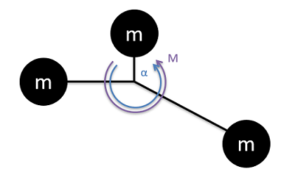
Taking our situation one step further, if we were to have multiple masses all connected to a central point, the moment and angular acceleration would be related by the sum of all the mass times distance squared terms.

\[ M = \sum (m * d^2) * \alpha \]

Three massless rods of different lengths radiate out from a single point, and each rod holds a point mass m on its free end. A counterclockwise moment is applied to the central point where the rods connect. — Figure \(\PageIndex{2}\): For systems with multiple masses, we would simply sum up all the mass-times-distance-squared terms to relate moments and angular accelerations.

Taking the final step, rigid bodies with mass distributed over a volume are like an infinite number of small masses about an axis of rotation. Rather than the massless sticks holding everything in place, the mass is simply held in place by the material around it. To relate the moment and angular acceleration in this case, we use integration to add up the infinite number of small mass-times-distance-squared terms.

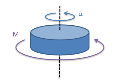
A vertical cylinder is rotated counterclockwise about its central axis. — Figure \(\PageIndex{3}\): Approximating a rigid body as an infinite number of infinitely small masses all connected to the axis of rotation, we can sum all the mass-times-distance-squared terms with integration.

\[ M = \int_m (dm * d^2) * \alpha \]

This moment integral which can be calculated for any given shape, called the mass moment of inertia, relates the moment and the angular acceleration for the body about a set axis of rotation.

\[ I = \int_m (dm * d^2) \]

Calculating the Mass Moment of Inertia via Integration

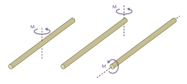
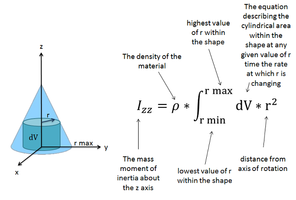
The first step in calculating the mass moment of inertia is to determine the axis of rotation you will be using. Unlike mass, the mass moment of inertia is dependent upon the point and axis that we are rotating about. We can easily demonstrate this with something like a broomstick, where depending on the position and the direction of the axis we are rotating about, the broomstick can be more or less difficult to rotate.

A broomstick in the same current orientation will have different mass moments of inertia depending on whether it is rotated about the midpoint of its length, about one end, or about its central axis. — Figure \(\PageIndex{4}\): The mass moment of inertia will vary depending upon the point and direction of the axis of rotation.

After choosing the axis of rotation, it is helpful to draw the shape with the axis of rotation included. This is a polar integral, so we will be taking the mass integral radiating outwards from this axis of rotation.

Also, we are integrating over the mass, and the mass at any given point will be the density times the volume. If the object we are examining has a uniform density, as is often the case, we can pull that density constant outside of the integral, leaving only a integral of the volume. Density is rarely given in these instances, but if you can determine the overall mass and overall volume you can use that as well. If we put all of this into the original equation we had above, we wind up with the following.

\[ I = \rho * \int_{r_{min}}^{r_{max}} (dV * r^2) = \frac{m}{V} * \int_{r_{min}}^{r_{max}} (dV * r^2) \]

For the polar integral, we need to define \(dV\) in terms of a radius (\(r\)) moving outwards from the axis of rotation. The rate of change of the volume (\(dV\)) will be the cylindrical surface area at a given radius times the rate at which that radius is increasing (\(dr\)). The height, radius, and holes in this cylindrical surface may all be changing so this \(dV\) term may become quite complex, but technically we could find this for mathematical function for any shape. Once we have the \(dV\) function in terms of \(r\), we multiply that function by \(r^2\) and we will evaluate the integral.

A cone with its base centered on the xy-plane of a Cartesian coordinate system and its height stretching upward along the positive z-axis is divided into thin cylindrical shells, each of a constant radius r measured from the z-axis. The volume of each of these shells is dV. The moment of inertia about the z-axis is the constant density rho times the integral of dV times r-squared, evaluated from the shape's minimum r-value to its maximum r-value. — Figure \(\PageIndex{5}\): The mass moment of inertia for a general shape.

Video lecture covering this section, delivered by Dr. Jacob Moore. YouTube source: https://youtu.be/uarIssOmWUU.

Example \(\PageIndex{1}\)

A thin circular disk has a mass of 6 kg and a radius of 0.3 meters. Determine the mass moment of inertia for the disk about the \(z\)-axis.

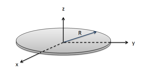
A thin cylindrical disk lies on the xy-plane of a three-dimensional Cartesian coordinae system, with the x-axis pointing out of the screen and the y-axis lying horizontally in the plane of the screen. The disk's base is centered on the origin, and the disk height stretches along the positive z-axis. — Figure \(\PageIndex{6}\): problem diagram for Example \(\PageIndex{1}\). A thin cylindrical disk lies along the \(z\)-axis with its base on the \(xy\)-plane, centered at the origin.

Solution:: Video \(\PageIndex{2}\): Worked solution to example problem \(\PageIndex{1}\), provided by Dr. Jacob Moore. YouTube source: https://youtu.be/e1ZDv6xDUV8.

Example \(\PageIndex{2}\)

Determine the mass moment of inertia about the \(z\)-axis for this general cone with base radius \(R\), height \(h\), and mass \(m\).

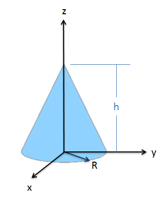
A three-dimensional Cartesian coordinate system, with the x-axis pointing out of the screen, the y-axis lying horizontally in the plane of the screen, and the z-axis lying vertically in the plane of the screen. A right circular cone lies with its base in the xy-plane, centered on the origin, and its height stretching along the positive z-axis. — Figure \(\PageIndex{7}\): problem diagram for Example \(\PageIndex{2}\). A cone lies along the positive \(z\)-axis, with the base centered at the origin in the \(xy\)-plane.

Solution:: Video \(\PageIndex{3}\): Worked solution to example problem \(\PageIndex{2}\), provided by Dr. Jacob Moore. YouTube source: https://youtu.be/rL7xWl9FfWc.