17.7: Moments of Inertia via Composite Parts and Parallel Axis Theorem

As an alternative to integration, both area and mass moments of inertia can be calculated via the method of composite parts, similar to what we did with centroids. In this method we will break down a complex shape into simple parts, look up the moments of inertia for these parts in a table, adjust the moments of inertia for position, and finally add the adjusted values together to find the overall moment of inertia. This method is known as the method of composite parts.

A key part to this process that was not present in centroid calculations is the adjustment for position. As discussed on the previous pages, the area and mass moments of inertia are dependent upon the chosen axis of rotation. Moments of inertia for the parts of the body can only be added when they are taken about the same axis. However, the moments of inertia in the table are generally listed relative to that shape's centroid. Because each part has its own individual centroid coordinate, we cannot simply add these numbers. We will use something called the Parallel Axis Theorem to adjust the moments of inertia so that they are all taken about some standard axis or point. Once the moments of inertia are adjusted with the Parallel Axis Theorem, then we can add them together using the method of composite parts.

The Parallel Axis Theorem

When we calculated the area and mass moments of inertia via integration, one of the first things we had to do was to select a point or axis we were going to take the moment of inertia about. We then measured all distances from that point or axis, where the distances were the moment arms in our moment integrals. Because the centroid of a shape is the geometric center of an area or volume, the average distance from the centroid to any one point in a body is at a minimum. If we pick a different point or axis to take the moment of inertia about, then on average all the distances in our moment integral will be a little bit bigger. Specifically, the further we move from the centroid, the larger the average distances become.

Figure \(\PageIndex{1}\): The distances used in our moment integrals depends on the point or axis chosen. These distances will be at a minimum at the centroid and will get larger as we move further from the centroid.

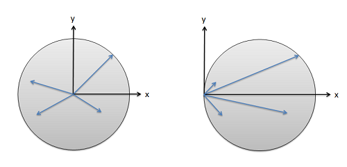
Though this complicates our analysis, the nice thing is that the change in the moment of inertia is predictable. It will always be at a minimum when we take the moment of inertia about the centroid, or an axis going through the centroid. This minimum, which we will call \(I_C\), is the value we will look up in our moment of inertia table. From this minimum, or unadjusted value, we can find the moment of inertia value about any point \(I_P\) by adding an an adjustment factor equal to the area times distance squared for area moments of inertia, or mass times distance squared for mass moments of inertia.

\[ I_{xxP} = I_{xxC} + A * r^2 \]

\[ I_{xxP} = I_{xxC} + m * r^2 \]

This adjustment process with the equations above is the parallel axis theorem. The area or mass terms simply represent the area or mass of the part you are looking at, while the distance (\(r\)) represents the distance that we are moving the axis about which we are taking the moment of inertia. This may be a vertical distance, a horizontal distance, or a diagonal depending on the axis the moment of inertia is taken about.

Figure \(\PageIndex{2}\): The distance (\(r\)) in the Parallel Axis Theorem represents the distance we are moving the axis we are taking the moment of inertia about.

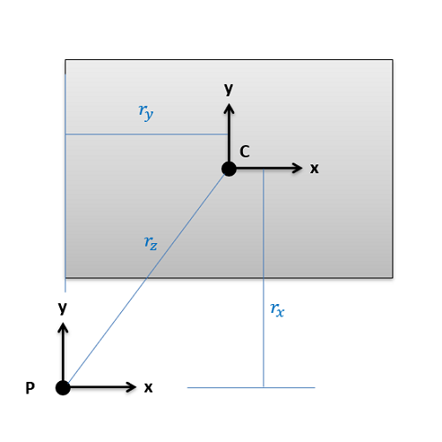
Say we are trying to find the moments of inertia of the rectangle above about point \(P\). We would start by looking up \(I_{xx}\), \(I_{yy}\), and \(J_{zz}\) about the centroid of the rectangle (\(C\)) in the moment of inertia table. Then we would add on an area-times-distance-squared term to each to find the adjusted moments of inertia about \(P\). The distance we are moving the \(x\) axis for \(I_{xx}\) is the vertical distance \(r_x\), the distance we are moving the \(y\)-axis for \(I_{yy}\) is the horizontal distance \(r_y\), and the distance we would move the \(z\)-axis (which is pointing out of the page) for \(J_{zz}\) is the diagonal distance \(r_z\).

Center of mass adjustments follow a similar logic, using mass times distance squared, where the distance represents how far you are moving the axis of rotation in three-dimensional space.

Using the Method of Composite Parts to Find the Moment of Inertia

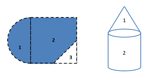
To find the moment of inertia of a body using the method of composite parts, you need to start by breaking your area or volume down into simple shapes. Make sure each individual shape is available in the moment of inertia table, and you can treat holes or cutouts as negative area or mass.

Figure \(\PageIndex{3}\): Start by breaking down your area or volume into simple parts, and number those parts. Holes or cutouts will count as negative areas or masses.

Next you are going to create a table to keep track of values. Devote a row to each part that your numbered earlier, and include a final "total" row that will be used for some values. Most of the work of the method of composite parts is filling in this table. The columns will vary slightly with what you are looking for, but you will generally need the following.

Figure \(\PageIndex{4}\): Most work in the method of composite parts will revolve around filling out a table such as this one. This table contains the rows and columns necessary to find the rectangular area moments of inertia (\(I_{xx}\) and \(I_{yy}\)) for this composite body.

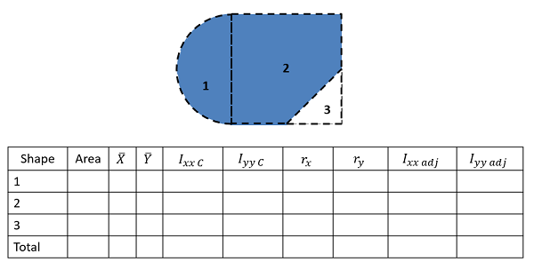
• The area or mass for each piece (area for area moments of inertia or mass for mass moments of inertia). Remember that cutouts should be listed as negative areas or masses.
• The centroid or center of mass locations (\(x\), \(y\) and possibly \(z\) coordinates). Most of the time, we will be finding the moment of inertia about centroid of the composite shape, and if that is not explicitly given to you, you will need to find that before going further. For more details on this, see the page Centroids and Centers of Mass via Method of Composite Parts.
• The moment of inertia values about each shape's centroid. To find these values you will plug numbers for height, radius, mass, etc. into formulas on the moment of inertia table. Do not use these formulas blindly though, as you may need to mentally rotate the body, and thus switch equations, if the orientation of the shape in the table does not match the orientation of the shape in your diagram.
• The adjustment distances (\(r\)) for each shape. For this value you will want to determine how far the \(x\)-axis, \(y\)-axis, or \(z\)-axis moves to go from the centroid of the piece to the overall centroid or point you are taking the moment of inertia about. To calculate these values, generally you will be finding the horizontal, vertical, or diagonal distances between piece centroids and the overall centroids that you have listed earlier in the table. See the parallel axis theorem section of this page earlier for more details.
• Finally, you will have a column of the adjusted moments of inertia. Take the original moment of inertia about the centroid, then simply add your area times \(r^2\) term or mass times \(r^2\) term for this adjusted value.

The overall moment of inertia of your composite body is simply the sum of all of the adjusted moments of inertia for the pieces, which will be the sum of the values in the last column (or columns, if you are finding the moments of inertia about more than one axis).

Video \(\PageIndex{1}\): Video lecture covering this section, delivered by Dr. Jacob Moore. YouTube source: https://youtu.be/zulGTSWF6xs.

Example \(\PageIndex{1}\)

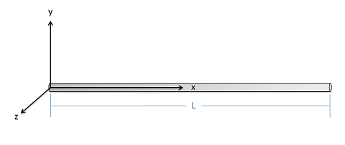
Use the parallel axis theorem to find the mass moment of inertia of this slender rod with mass \(m\) and length \(L\) about the \(z\)-axis at its endpoint.

Figure \(\PageIndex{5}\): problem diagram for Example \(\PageIndex{1}\). A rod lies along the positive \(x\)-axis of a Cartesian coordinate system, with its left endpoint located at the origin.

Solution:

Video \(\PageIndex{2}\): Worked solution to example problem \(\PageIndex{1}\), provided by Dr. Jacob Moore. YouTube source: https://youtu.be/4oN0kgDO3Yw.

Example \(\PageIndex{2}\)

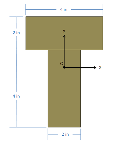
A beam is made by connecting two 2" x 4" beams in a T-pattern with the cross section as shown below. Determine the location of the centroid of this combined cross section and then find the rectangular area moment of inertia about the \(x\)-axis through the centroid point.

Figure \(\PageIndex{6}\): problem diagram for Example \(\PageIndex{2}\). The top edge of a vertical 2" x 4" beam is centered on and connected to the lower edge of a horizontal 2" x 4" beam, creating a T-shaped assembly.

Solution:

Video \(\PageIndex{3}\): Worked solution to example problem \(\PageIndex{2}\), provided by Dr. Jacob Moore. YouTube source: https://youtu.be/lgXlp2lRaiA.

Example \(\PageIndex{3}\)

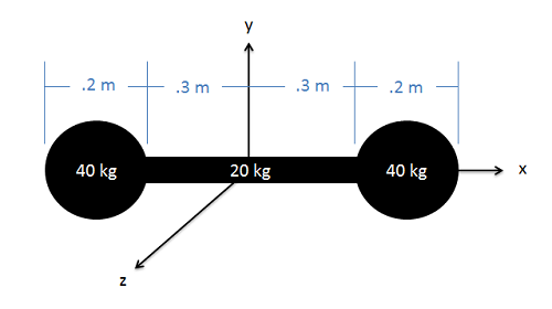
A dumbbell consists of two spheres of diameter 0.2 meter, each with a mass of 40 kg, attached to the ends of a 0.6-meter-long slender rod of mass 20 kg. Determine the mass moment of inertia of the dumbbell about the \(y\)-axis shown in the diagram.

Figure \(\PageIndex{7}\): problem diagram for Example \(\PageIndex{3}\). A dumbbell consists of a slender rod with a sphere attached to each end lying along the \(x\)-axis of a Cartesian coordinate system, with its midpoint at the origin.

Solution:

Video \(\PageIndex{4}\): Worked solution to example problem \(\PageIndex{3}\), provided by Dr. Jacob Moore. YouTube source: https://youtu.be/ufewJ7CmvIs.