1.3: Introduction to Composites

Introduction

This module introduces basic concepts of stiffness and strength underlying the mechanics of fiber-reinforced advanced composite materials. This aspect of composite materials technology is sometimes terms \micromechanics," because it deals with the relations between macroscopic engineering properties and the microscopic distribution of the material's constituents, namely the volume fraction of fiber. This module will deal primarily with unidirectionally-reinforced continuous-fiber composites, and with properties measured along and transverse to the fiber direction.

Materials

The term composite could mean almost anything if taken at face value, since all materials are composed of dissimilar subunits if examined at close enough detail. But in modern materials engineering, the term usually refers to a "matrix" material that is reinforced with fibers. For in- stance, the term "FRP" (for Fiber Reinforced Plastic) usually indicates a thermosetting polyester matrix containing glass fibers, and this particular composite has the lion's share of today's commercial market. Figure 1 shows a laminate fabricated by "crossplying" unidirectionally-reinforced layers in a \(0^{\circ}-90^{\circ}\) stacking sequence.

Many composites used today are at the leading edge of materials technology, with performance and costs appropriate to ultrademanding applications such as spacecraft. But heterogeneous materials combining the best aspects of dissimilar constituents have been used by nature for millions of years. Ancient society, imitating nature, used this approach as well: the Book of Exodus speaks of using straw to reinforce mud in brickmaking, without which the bricks would have almost no strength.

As seen in Table 1(F.P. Gerstle, "Composites," Encyclopedia of Polymer Science and Engineering, Wiley, New York, 1991. Here \(E\) is Young's modulus, \(\sigma_b\) is breaking stress, \(\epsilon_b\) is breaking strain, and \(\rho\) is density.), the fibers used in modern composites have strengths and stiffnesses far above those of traditional bulk materials. The high strengths of the glass fibers are due to processing that avoids the internal or surface flaws which normally weaken glass, and the strength and stiffness of the polymeric aramid fiber is a consequence of the nearly perfect alignment of the molecular chains with the fiber axis.

Figure 1: A crossplied FRP laminate, showing nonuniform fiber packing and microcracking (from Harris, 1986).

Table 1: Properties of Composite Reinforcing Fibers.

Material	\(E\) (GPa)	\(\sigma_b\) (GPa)	\(\epsilon_b\) (%)	\(\rho\) \(Mg/m^3\)	\(E/\rho\) \((MJ/kg)\)	\(\sigma_b /\rho\) \((MJ/kg)\)	cost ($/kg)
E-glass	72.4	2.4	2.6	2.54	28.5	0.95	1.1
S-glass	85.5	4.5	2.0	2.49	34.3	1.8	22-33
aramid	124	3.6	2.3	1.45	86	2.5	22-33
boron	400	3.5	1.0	2.45	163	1.43	33-440
HS graphite	253	4.5	1.1	1.80	140	2.5	66-110
HM graphite	520	2.4	0.6	1.85	281	1.3	220-660

Of course, these materials are not generally usable as fibers alone, and typically they are impregnated by a matrix material that acts to transfer loads to the fibers, and also to protect the fibers from abrasion and environmental attack. The matrix dilutes the properties to some degree, but even so very high specific (weight-adjusted) properties are available from these materials. Metal and glass are available as matrix materials, but these are currently very expensive and largely restricted to R&D laboratories. Polymers are much more commonly used, with unsaturated styrene-hardened polyesters having the majority of low-to-medium performance applications and epoxy or more sophisticated thermosets having the higher end of the market. Thermoplastic matrix composites are increasingly attractive materials, with processing difficulties being perhaps their principal limitation.

Stiffness

The fibers may be oriented randomly within the material, but it is also possible to arrange for them to be oriented preferentially in the direction expected to have the highest stresses. Such a material is said to be anisotropic (different properties in different directions), and control of the anisotropy is an important means of optimizing the material for specific applications. At a microscopic level, the properties of these composites are determined by the orientation and distribution of the fibers, as well as by the properties of the fiber and matrix materials. The topic known as composite micromechanics is concerned with developing estimates of the overall material properties from these parameters.

Figure 2: Loading parallel to the fibers.

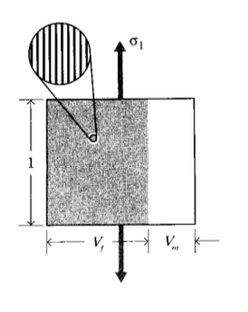
Consider a typical region of material of unit dimensions, containing a volume fraction \(V-f\) of fibers all oriented in a single direction. The matrix volume fraction is then \(V_m = 1 - V_f\). This region can be idealized as shown in Figure 2 by gathering all the fibers together, leaving the matrix to occupy the remaining volume -- this is sometimes called the "slab model." If a stress \(\sigma_1\) is applied along the fiber direction, the fiber and matrix phases act in parallel to support the load. In these parallel connections the strains in each phase must be the same, so the strain \(\epsilon_1\) in the fiber direction can be written as:

\[\epsilon_f = \epsilon_m = \epsilon_1\nonumber\]

The forces in each phase must add to balance the total load on the material. Since the forces in each phase are the phase stresses times the area (here numerically equal to the volume fraction), we have

\[\sigma_1 = \sigma_f V_f + \sigma_m V_m = E_f \epsilon_1 V_f + E_m \epsilon_1 V_m\nonumber\]

The stiffness in the fiber direction is found by dividing by the strain:

\[E_1 = \dfrac{\sigma_1}{\epsilon_1} = V_f E_f + V_m E_m\]

This relation is known as a rule of mixtures prediction of the overall modulus in terms of the moduli of the constituent phases and their volume fractions.

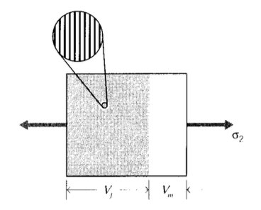
If the stress is applied in the direction transverse to the fibers as depicted in Figure 3, the slab model can be applied with the fiber and matrix materials acting in series. In this case the stress in the fiber and matrix are equal (an idealization), but the defflections add to give the overall transverse deflection. In this case it can be shown (see Exercise \(\PageIndex{5}\))

\[\dfrac{1}{E_2} = \dfrac{V_f}{E_f} + \dfrac{V_m}{E_m}\]

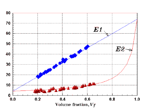
Figure 4 shows the functional form of the parallel (Equation 1.3.1) and series (Equation 1.3.2) predictions for the fiber- and transverse-direction moduli.

Figure 3: Loading perpendicular to the fibers.

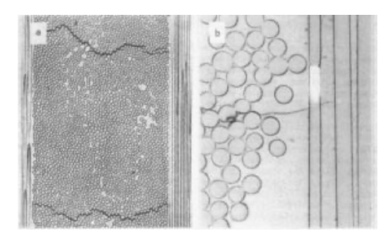
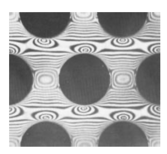
The prediction of transverse modulus given by the series slab model (Equation 1.3.2) is considered unreliable, in spite of its occasional agreement with experiment. Among other deficiencies the assumption of uniform matrix strain being untenable; both analytical and experimental studies have shown substantial nonuniformity in the matirx strain. Figure 5 shows the photoelastic fringes in the matrix caused by the perturbing effect of the stiffer fibers. (A more complete description of these phtoelasticity can be found in the Module on Experimental Strain Analysis, but this figure can be interpreted simply by noting that closely-spaced photoelastic fringes are indicative of large strain gradients.

In more complicated composites, for instance those with fibers in more than one direction or those having particulate or other nonfibrous reinforcements, Equation 1.3.1 provides an upper bound to the composite modulus, while Equation 1.3.2 is a lower bound (see Figure 4). Most practical cases will be somewhere between these two values, and the search for reasonable models for these intermediate cases has occupied considerable attention in the composites research community. Perhaps the most popular model is an empirical one known as the Halpin-Tsai equation(c.f. J.C.. Halpin and J.L. Kardos, Polymer Engineering and Science, Vol. 16, May 1976, pp. 344{352.), which can be written in the form:

\[E = \dfrac{E_m[E_f + \xi (V_f E_f + V_m E_m)]}{V_f E_m + V_m E_f + \xi E_m}\]

Here \(\xi\) is an adjustable parameter that results in series coupling for \(\xi = 0\) and parallel averaging for very large \(\xi\).

Strength

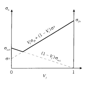
Rule of mixtures estimates for strength proceed along lines similar to those for stiffness. For instance, consider a unidirectionally reinforced composite that is strained up to the value at which the fibers begin to break. Denoting this value \(\epsilon_{fb}\), the stress transmitted by the composite is given by multiplying the stiffness (Equation 1.3.1):

\[\sigma_b = \epsilon_{fb} E_1 = V_f \sigma_{fb} + (1 - V_f) \sigma^*\nonumber\]

Figure 4: Rule-of-mixtures predictions for longitudinal (\(E_1\)) and transverse (\(E_2\)) modulus, for glass-polyester composite (\(E_f = 73.7\) MPa, \(E_m = 4\) GPa). Experimental data taken from Hull (1996).

The stress \(\sigma^*\) is the stress in the matrix, which is given by \(\epsilon_{fb} E_m\). This relation is linear in \(V_f\), rising from \(\sigma^*\) to the fiber breaking strength \(\sigma_{fb} = E_f \epsilon_{fb}\). However, this relation is not realistic at low fiber concentration, since the breaking strain of the matrix \(\epsilon_{mb}\) is usually substantially greater than \(\epsilon_{fb}\). If the matrix had no fibers in it, it would fail at a stress \(\sigma_{mb} = E_m \epsilon_{mb}\). If the fibers were considered to carry no load at all, having broken at \(\epsilon = \epsilon_{fb}\) and leaving the matrix to carry the remaining load, the strength of the composite would fall off with fiber fraction according to

\[\sigma_b = (1 - V_f) \sigma_{mb}\nonumber\]

Since the breaking strength actually observed in the composite is the greater of these two expressions, there will be a range of fiber fraction in which the composite is weakened by the addition of fibers. These relations are depicted in Figure 6.

References

1. Ashton, J.E., J.C. Halpin and P.H. Petit, Primer on Composite Materials: Analysis,Technomic Press, Westport, CT, 1969.
2. , Harris, B., Engineering Composite Materials, The Institute of Metals, London, 1986.
3. Hull, D. and T.W. Clyne, An Introduction to Composites Materials, Cambridge University

   Press, 1996.

4. Jones, R.M., Mechanics of Composite Materials, McGraw-Hill, New York, 1975.
5. Powell, P.C, Engineering with Polymers, Chapman and Hall, London, 1983.
6. Roylance, D., Mechanics of Materials, Wiley & Sons, New York, 1996.

Figure 5: Photoelastic (isochromatic) fringes in a composite model subjected to transverse tension (from Hull, 1996).

Figure 6: Strength of unidirectional composite in fiber direction.

Exercise \(\PageIndex{1}\)

Compute the longitudinal and transverse stiffness (\(E_1,E_2\)) of an S-glass epoxy lamina for a fiber volume fraction \(V_f = 0.7\), using the fiber properties from Table 1, and matrix properties from the Module on Materials Properties.

Exercise \(\PageIndex{2}\)

Plot the longitudinal stiffness \(E_1\) of an E-glass/nylon unidirectionally-reinforced composite, as a function of the volume fraction \(V_f\).

Exercise \(\PageIndex{3}\)

Plot the longitudinal tensile strength of a E-glass/epoxy unidirectionally-reinforced composite, as a function of the volume fraction \(V_f\)

Exercise \(\PageIndex{4}\)

What is the maximum fiber volume fraction \(V_f\) that could be obtained in a unidirectionally reinforced with optimal fiber packing?

Exercise \(\PageIndex{5}\)

Using the slab model and assuming uniform strain in the matrix, show the transverse modulus of a unidirectionally-reinforced composite to be

\[\dfrac{1}{E_2} = \dfrac{V_f}{E_f} + \dfrac{V_m}{E_m}\nonumber\]

or in terms of compliances

\[C_2 = C_f V_f + C_m V_m\nonumber\]