
3.3: Tensor Transformations
- Page ID
- 44537

Introduction
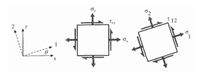
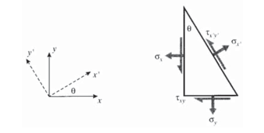
One of the most common problems in mechanics of materials involves transformation of axes. For instance, we may know the stresses acting on \(xy\) planes, but are really more interested in the stresses acting on planes oriented at, say, 30\(^{\circ}\) to the \(x\) axis as seen in Figure 1, perhaps because these are close-packed atomic planes on which sliding is prone to occur, or is the angle at which two pieces of lumber are glued together in a "scarf" joint. We seek a means to transform the stresses to these new \(x'y'\) planes.
These transformations are vital in analyses of stress and strain, both because they are needed to compute critical values of these entities and also because the tensorial nature of stress and strain is most clearly seen in their transformation properties. Other entities, such as moment of inertia and curvature, also transform in a manner similar to stress and strain. All of these are second-rank tensors, an important concept that will be outlined later in this module.
Direct approach
The rules for stress transformations can be developed directly from considerations of static equilibrium. For illustration, consider the case of uniaxial tension shown in Figure 2 in which all stresses other than \(\sigma_y\) are zero. A free body diagram is then constructed in which the specimen is "cut" along the inclined plane on which the stresses, labeled \(\sigma_{y'}\) and \(\tau_{x'y'}\), are desired. The key here is to note that the area on which these transformed stresses act is different than the area normal to the y axis, so that both the areas and the forces acting on them need to be "transformed." Balancing forces in the \(y'\) direction (the direction normal to the inclined plane):
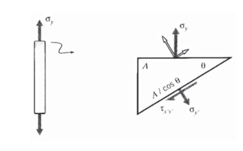
\((\sigma_y A) \cos \theta = \sigma_{y'} \left (\dfrac{A}{\cos \theta} \right )\)
\[\sigma_{y'} = \sigma_y \cos^2 \theta\]
Similarly, a force balance in the tangential direction gives
\[\tau_{x'y'} = \sigma_y \sin \theta \cos \theta\]
Example \(\PageIndex{1}\)
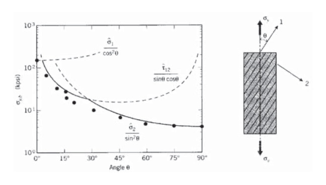
Consider a unidirectionally reinforced composite ply with strengths \(\hat{\sigma}_1\) in the fiber direction, \(\hat{\sigma}_2\) in the transverse direction, and \(\hat{\tau}_{12}\) in shear. As the angle \(\theta\) between the fiber direction and an applied tensile stress \(\sigma_y\) is increased, the stress in the fiber direction will decrease according to Equation 3.3.1. If the ply were to fail by fiber fracture alone, the stress \(\sigma_{y, b}\) needed to cause failure would increase with misalignment according to \(\sigma_{y, b} = \hat{\sigma}_1/\cos^2 \theta\).
However, the shear stresses as given by Equation 3.3.2 increase with \(\theta\), so the σy stress needed for shear failure drops. The strength \(\sigma_{y,b}\) is the smaller of the stresses needed to cause fiber-direction or shear failure, so the strength becomes limited by shear after only a few degrees of misalignment. In fact, a 15\(^{\circ}\) off-axis tensile specimen has been proposed as a means of measuring intralaminar shear strength. When the orientation angle approaches 90\(^{\circ}\), failure is dominated by the transverse strength. The experimental data shown in Figure 3 are for glass-epoxy composites(R.M. Jones, Mechanics of Composite Materials, McGraw-Hill, 1975.), which show good but not exact agreement with these simple expressions.
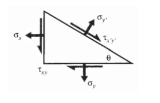
A similar approach, but generalized to include stresses \(\sigma_x\) and \(\tau_{xy}\) on the original \(xy\) planes as shown in Figure 4 (see Exercise \(\PageIndex{2}\)) gives:
\[\begin{array} {rcl} {\sigma_{x'}} & = & {\sigma_x \cos^2 \theta + \sigma_y \sin^2 \theta + 2 \tau_{xy} \sin \theta \cos \theta} \\ {\sigma_{y'}} & = & {\sigma_x \sin^2 \theta + \sigma_y \cos^2 \theta - 2 \tau_{xy} \sin \theta \cos \theta} \\ {\tau_{x'y'}} & = & {(\sigma_y - \sigma_x) \sin \theta \cos \theta + \tau_{xy} (\cos^2 \theta - \sin^2 \theta)} \end{array}\]
These relations can be written in pseudovector-matrix form as
\[\left \{\begin{array} {c} {\sigma_{x'}} \\ {\sigma_{y'}} \\ {\tau_{x'y'}} \end{array} \right \} = \begin{bmatrix} c^2 & s^2 & 2sc \\ s^2 & c^2 & -2sc \\ -sc & sc & c^2 - s^2 \end{bmatrix} \left \{\begin{array} {c} {\sigma_{x}} \\ {\sigma_{y}} \\ {\tau_{xy}} \end{array} \right \}\]
where \(c = \cos \theta\) and \(s = \sin \theta\). This can be abbreviated as
\[\sigma'=A \sigma\]
where \(A\) is the transformation matrix in brackets above. This expression would be valid for three dimensional as well as two dimensional stress states, although the particular form of \(A\) given in Equation 3.3.4 is valid in two dimensions only (plane stress), and for Cartesian coordinates.
Using either mathematical or geometric arguments (see Exercise \(\PageIndex{3}\) and Exercise \(\PageIndex{4}\)), it can be shown that the components of infinitesimal strain transform by almost the same relations:
\[\left \{\begin{array} {c} {\sigma_{x'}} \\ {\sigma_{y'}} \\ {\dfrac{1}{2} \gamma_{x'y'}} \end{array} \right \} = A \left \{\begin{array} {c} {\sigma_{x}} \\ {\sigma_{y}} \\ {\dfrac{1}{2} \gamma_{xy}} \end{array} \right \}\]
The factor of 1/2 on the shear components arises from the classical definition of shear strain, which is twice the tensorial shear strain. This introduces some awkwardness into the transformation relations, some of which can be reduced by defining the Reuter’s matrix as
\[[R] = \begin{bmatrix} 1 & 0 & 0 \\ 0 & 1 & 0 \\ 0 & 0 & 2 \end{bmatrix} \ \ or \ \ [R]^{-1} = \begin{bmatrix} 1 & 0 & 0 \\ 0 & 1 & 0 \\ 0 & 0 & \tfrac{1}{2} \end{bmatrix}\]
We can now write:
\[\left \{\begin{array} {c} {\sigma_{x'}} \\ {\sigma_{y'}} \\ {\gamma_{x'y'}} \end{array} \right \} = R \left \{\begin{array} {c} {\sigma_{x'}} \\ {\sigma_{y'}} \\ {\dfrac{1}{2} \gamma_{x'y'}} \end{array} \right \} = RA \left \{\begin{array} {c} {\sigma_{x}} \\ {\sigma_{y}} \\ {\dfrac{1}{2} \gamma_{xy}} \end{array} \right \} = RAR^{-1} \left \{\begin{array} {c} {\sigma_{x}} \\ {\sigma_{y}} \\ {\gamma_{xy}} \end{array} \right \} \nonumber\]
Or
\[\epsilon' = RAR^{-1} \epsilon\]
As can be verified by expanding this relation, the transformation equations for strain can also be obtained from the stress transformation equations (e.g. Equation 3.3.3) by replacing \(\sigma\) with \(\epsilon\) and \(\tau\) with \(\gamma /2\):
\[\begin{array} {rcl} {\epsilon_{x'}} & = & {\epsilon_x \cos^2 \theta + \epsilon_y \sin^2 \theta + \gamma_{xy} \sin \theta \cos \theta} \\ {\epsilon_{y'} & = & {\epsilon_x \sin^2 \theta + \epsilon_y \cos^2 \theta - \gamma_{xy} \sin \theta \cos \theta} \\ {\gamma_{x'y'}} & = & {2 (\epsilon_y - \epsilon_x) \sin \theta \cos \theta + \gamma_{xy} (\cos^2 \theta - \sin^2 \theta)} \end{array}\]
Example \(\PageIndex{2}\)
Consider the biaxial strain state
\[\epsilon = \left \{\begin{array} {c} {\sigma_{x'}} \\ {\sigma_{y'}} \\ {\gamma_{x'y'}} \end{array} \right \} = \left \{\begin{array} {c} {0.01} \\ {-0.01} \\ {0} \end{array} \right \} \nonumber\]
The state of strain \(\epsilon'\) referred to axes rotated by \(\theta = 45^{\circ}\) from the \(x-y\) axes can be computed by matrix multiplication as:
\[A = \begin{bmatrix} c^2 & s^2 & 2sc \\ s^2 & c^2 & -2sc \\ -sc & sc & c^2 - s^2 \end{bmatrix} = \begin{bmatrix} 0.5 & 0.5 & 1.0 \\ 0.5 & 0.5 & -1.0 \\ -0.5 & 0.5 & 0.0 \end{bmatrix} \nonumber\]
Then
\[\epsilon' = RAR^{-1} \epsilon \nonumber\]
\[\begin{bmatrix} 1.0 & 1.0 & 0.0 \\ 0.0 & 1.0 & 0.0 \\ 0.0 & 0.0 & 2.0 \end{bmatrix} \begin{bmatrix} 0.5 & 0.5 & 1.0 \\ 0.5 & 0.5 & -1.0 \\ -0.5 & 0.5 & 0.0 \end{bmatrix} \begin{bmatrix} 1.0 & 0.0 & 0.0 \\ 0.0 & 1.0 & 0.0 \\ 0.0 & 0.0 & 0.5 \end{bmatrix} = \left \{\begin{array} {c} {0.00} \\ {0.00} \\ {-0.02} \end{array} \right \}\nonumber\]
Obviously, the matrix multiplication method is tedious unless matrix-handling software is available, in which case it becomes very convenient.
Mohr’s circle
Everyday experience with such commonplace occurrences as pushing objects at an angle gives us all a certain intuitive sense of how vector transformations work. Second-rank tensor transformations seem more abstract at first, and a device to help visualize them is of great value. As it happens, the transformation equations have a famous (among engineers) graphical interpretation known as Mohr's circle(Presented in 1900 by the German engineer Otto Mohr (1835–1918).). The Mohr procedure is justified mathematically by using the trigonometric double-angle relations to show that Eqns. 3.3.3 have a circular representation (see Exercise \(\PageIndex{5}\)), but it can probably best be learned simply by memorizing the following recipe(An interactive web demonstration of Mohr’s circle construction is available at <http://web.mit.edu/course/3/3.11/www/java/mohr.html>.).
- Draw the stress square, noting the values on the x and y faces; Figure 5(a) shows a hypothetical case for illustration. For the purpose of Mohr’s circle only, regard a shear stress acting in a clockwise-rotation sense as being positive, and counter-clockwise as negative. The shear stresses on the \(x\) and \(y\) faces must then have opposite signs. The normal stresses are positive in tension and negative in compression, as usual.
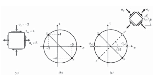
- Construct a graph with \(\tau\) as the ordinate (\(y\) axis) and \(\sigma\) as abscissa, and plot the stresses on the \(x\) and \(y\) faces of the stress square as two points on this graph. Since the shear stresses on these two faces are the negative of one another, one of these points will be above the σ-axis exactly as far as the other is below. It is helpful to label the two points as \(x\) and \(y\).
- Connect these two points with a straight line. It will cross the \(\sigma\) axis at the line’s midpoint. This point will be at \((\sigma_x + \sigma_y)/2\), which in our illustration is [5 + (−3)]/2 = 1.
- Place the point of a compass at the line’s midpoint, and set the pencil at the end of the line. Draw a circle with the line as a diameter. The completed circle for our illustrative stress state is shown in Figure 5(b).
- To determine the stresses on a stress square that has been rotated through an angle \(\theta\) with respect to the original square, rotate the diametral line in the same direction through twice this angle; i.e. \(2\theta\). The new end points of the line can now be labeled \(x'\) and \(y'\), and their \(\sigma - \tau\) values are the stresses on the rotated \(x'-y'\)axes as shown in Figure 5(c).
There is nothing mysterious or magical about the Mohr’s circle; it is simply a device to help visualize how stresses and other second-rank tensors change when the axes are rotated.
It is clear in looking at the Mohr’s circle in Figure 5(c) that there is something special about axis rotations that cause the diametral line to become either horizontal or vertical. In the first case, the normal stresses assume maximal values and the shear stresses are zero. These normal stresses are known as the principal stresses, \(\sigma_{p1}\) and \(\sigma_{p2}\), and the planes on which they act are the principal planes. If the material is prone to fail by tensile cracking, it will do so by cracking along the principal planes when the value of \(\sigma_{p1}\) exceeds the tensile strength.
Example \(\PageIndex{3}\)
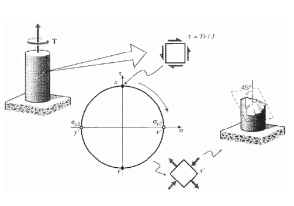
It is instructive to use a Mohr’s circle construction to predict how a piece of blackboard chalk will break in torsion, and then verify it in practice. The torsion produces a state of pure shear as shown in Figure 6, which causes the principal planes to appear at \(\pm 45^{\circ}\) to the chalk’s long axis. The crack will appear transverse to the principal tensile stress, producing a spiral-like failure surface. (As the crack progresses into the chalk, the state of pure shear is replaced by a more complicated stress distribution, so the last part of the failure surface deviates from this ideal path to one running along the axial direction.) This is the same type of fracture that occurred all too often in skiers’ femurs, before the advent of modern safety bindings.
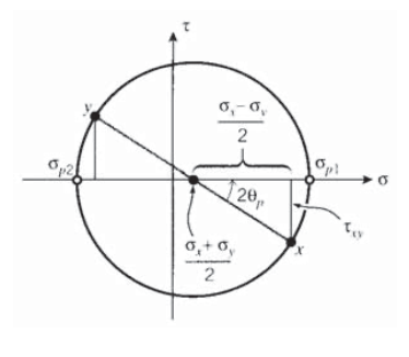
By direct Pythagorean construction as shown in Figure 7, the Mohr’s circle shows that the angle from the \(x-y\) axes to the principal planes is
\[\tan 2 \theta_p = \dfrac{\tau_{xy}}{(\sigma_x - \sigma_y)/2}\]
and the values of the principal stresses are
\[\sigma_{p1,p1} = \dfrac{\sigma_x + \sigma_y}{2} \pm \sqrt{(\dfrac{\sigma_x - \sigma_y}{2})^2 + \tau_{xy}^2}\]
where the first term above is the \(\sigma\)-coordinate of the circle’s center, and the second is its radius.
When the Mohr’s circle diametral line is vertical, the shear stresses become maximum, equal in magnitude to the radius of the circle:
\[\tau_{\max} = \sqrt{(\dfrac{\sigma_x - \sigma_y}{2})^2 + \tau_{xy}^2} = \dfrac{\sigma_{p1} - \sigma_{p2}}{2}\]
The points of maximum shear are 90\(^{\circ}\) away from the principal stress points on the Mohr’s circle, so on the actual specimen the planes of maximum shear are 45\(^{\circ}\) from the principal planes. The molecular sliding associated with yield is driven by shear, and usually takes place on the planes of maximum shear. A tensile specimen has principal planes along and transverse to its loading direction, so shear slippage will occur on planes \(\pm\)45\(^{\circ}\) from the loading direction. These slip planes can often be observed as "shear bands" on the specimen.
Note that normal stresses may appear on the planes of maximum shear, so the situation is not quite the converse of the principal planes, on which the shear stresses vanish while the normal stresses are maximum. If the normal stresses happen to vanish on the planes of maximum shear, the stress state is said to be one of "pure shear," such as is induced by simple torsion. A state of pure shear is therefore one for which a rotation of axes exists such that the normal stresses vanish, which is possible only if the center of the Mohr’s circle is at the origin, i.e. \((\sigma_x + \sigma_y)/2 = 0\). More generally, a state of pure shear is one in which the trace of the stress (and strain) matrix vanishes.
Example \(\PageIndex{4}\)
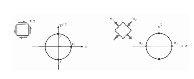
Mohr’s circles can be drawn for strains as well as stresses, with shear strain plotted on the ordinate and normal strain on the abscissa. However, the ordinate must be \(\gamma/2\) rather than just \(\gamma\), due to the way classical infinitesimal strains are defined. Consider a state of pure shear with strain \(\gamma\) and stress \(\tau\) as shown in Figure 8, such as might be produced by placing a circular shaft in torsion. A Mohr’s circle for strain quickly shows the principal strain, on a plane 45\(^{\circ}\) away, is given by \(\epsilon_1 = \gamma/2\). Hooke’s law for shear gives \(\tau = G \gamma\), so \(\epsilon_1 = \tau /2G\). The principal strain is also related to the principal stresses by
\[\epsilon_1 = \dfrac{1}{E} (\sigma_2 - \nu \sigma_2)\nonumber\]
The Mohr’s circle for stress gives \(\sigma_1 = -\sigma_2 = \tau\), so this can be written
\[\dfrac{\tau}{2G} = \dfrac{1}{E} [\tau - \nu (-\tau)]\nonumber\]
Canceling \(\tau\) and rearranging, we have the relation among elastic constants stated earlier without proof:
\[G = \dfrac{E}{2(1 + \nu)} \nonumber\]
General approach
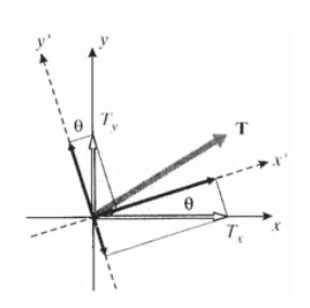
Another approach to the stress transformation equations, capable of easy extension to three dimensions, starts with the familiar relations by which vectors are transformed in two dimensions (see Figure 9):
\[T_{x'} = T_x \cos \theta + T_y \sin \theta \nonumber\]
\[T_{y'} = -T_x \sin \theta + T_y \cos \theta \nonumber\]
In matrix form, that is
\[\left \{ \begin{array} {c} {T_{x'}} \\ {T_{y'}} \end{array} \right \} = \begin{bmatrix} \cos \theta & \sin \theta \\ - \sin \theta & \cos \theta \end{bmatrix} \left \{ \begin{array} {c} {T_{x}} \\ {T_{y}} \end{array} \right \} \nonumber\]
or
\[T' = aT\]
where a is another transformation matrix that serves to transform the vector components in the original coordinate system to those in the primed system. In index-notation terms, this could also be denoted \(a_{ij}\), so that
\[T_i' = a_{ij} T_j\nonumber\]
The individual elements of aij are the cosines of the angles between the \(i^{th}\) primed axis and the \(j^{th}\) unprimed axis.
It can be shown by direct examination that the a matrix has the useful property that its inverse equals its transpose; i.e., \(a^{-1} = a^T\). We can multiply Equation 3.3. 13 by \(a^T\) to give
\[a^T T' = (a^T a) T = T\]
so the transformation can go from primed to unprimed, or the reverse.
These relations can be extended to yield an expression for transformation of stresses (or strains, or moments of inertia, or other similar quantities). Recall Cauchy’s relation in matrix form:
\[[\sigma] \hat{n} = T\nonumber\]
Using Equation 3.3.14 to transform the \(\hat{n}\) and \(T\) vectors into their primed counterparts, we have
\[[\sigma] a^T \hat{n}' = a^T T'\nonumber\]
Multiplying through by a:
\((a[\sigma] a^T) \hat{n}' = (aa^T) T' = T'\nonumber\]
This is just Cauchy’s relation again, but in the primed coordinate frame. The quantity in parentheses must therefore be \([\sigma']\):
\[[\sigma'] = a[\sigma] a^T\]
Therefore, transformation of stresses and can be done by pre- and postmultiplying by the same transformation matrix applicable to vector transformation. This can also be written out using index notation, which provides another illustration of the transformation differences between scalars (zero-rank tensors), vectors (first-rank tensors), and second-rank tensors:
\[\begin{array} {rcl} {\text{rank 0:}} & \ \ \ & {b' = b} \\ {\text{rank 1:}} & \ \ \ & {T_i' = a_{ij} T_j} \\ {\text{rank 2:}} & \ \ \ & {\sigma_{ij}' = a_{ij} a_{kl} \sigma_{kl}} \end{array}\]
In practical work, it is not always a simple matter to write down the nine elements of the a matrix needed in Equation 3.3.15. The squares of the components of \(\hat{n}\) for any given plane must sum to unity, and in order for the three planes of the transformed stress cube to be mutually perpendicular the dot product between any two plane normals must vanish. So not just any nine numbers will make sense. Obtaining a is made much easier by using "Euler angles" to describe axis transformations in three dimensions.
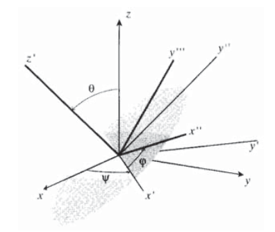
As shown in Figure 10, the final transformed axes are visualized as being achieved in three steps: first, rotate the original \(x-y-z\) axes by an angle \(\psi\) (psi) around the \(z\)-axis to obtain a new frame we may call \(x'-y'-z\). Next, rotate this new frame by an angle \(\theta\) about the \(x'\) axis to obtain another frame we can call \(x'-y''-z'\). Finally, rotate this frame by an angle \(\phi\) (phi) around the \(z'\) axis to obtain the final frame \(x''-y'''-z'\). These three transformations correspond to the transformation matrix
\[a = \begin{bmatrix} \cos \psi & \sin \psi & 0 \\ -\sin \psi & \cos \psi & 0 \\ 0 & 0 & 1 \end{bmatrix} \begin{bmatrix} 1 & 0 & 0 \\ 0 & \cos \theta & \sin \theta \\ 0 & -\sin \theta & \cos \theta \end{bmatrix} \begin{bmatrix} \cos \phi & \sin \phi & 0 \\ -\sin \phi & \cos \phi & 0 \\ 0 & 0 & 1 \end{bmatrix} \nonumber\]
This multiplication would certainly be a pain if done manually, but is a natural for a computational approach.
Example \(\PageIndex{5}\)
The output below shows a computer evaluation of a three-dimensional stress transformation, in this case using MapleTM symbolic mathematics software.
# read linear algebra library
> with(linalg):
# Define Euler-angle transformation matrices:
> a1:=array(1..3,1..3,[[cos(psi),sin(psi),0],[-sin(psi),cos(psi),0],[0,0 > ,1]]);
                      [cos(psi)     sin(psi)         0]
                a1 := [-sin(psi)    cos(psi)         0]
                      [   0              0           1]
> a2:=array(1..3,1..3,[[1,0,0],[0,cos(theta),sin(theta)],[0,-sin(theta),
> cos(theta)]]);
                      [1       0             0.   ]
                a2 := [0   cos(theta)   sin(theta)]
                      [0.  -sin(theta)  cos(theta)]
> a3:=array(1..3,1..3,[[cos(phi),sin(phi),0],[-sin(phi),cos(phi),0],[0,0 > ,1]]);
                      [cos(phi)     sin(phi)     0]
                a3 := [-sin(phi)    cos(phi)     0]
                      [    0             0       1]
# Overall transformation matrix (multiply individual Euler matrices):
> a:=a1&*a2&*a3;
                       a := (a1 &* a2) &* a3
# Set precision and read in Euler angles (converted to radians); here
# we are rotating 30 degrees around the z axis only.
> Digits:=4;psi:=0;theta:=30*(Pi/180);phi:=0;
                             Digits := 4
                               psi := 0
                          theta := 1/6 Pi
                               phi := 0
# Display transformation matrix for these angles: "evalf" evaluates the
# matrix element, and "map" applies the evaluation to each element of
# the matrix.
> aa:=map(evalf,evalm(a));
                        [1.      0.      0.  ]
                  aa := [0.    .8660    .5000]
                        [0.   -.5000    .8660]
# Define the stress matrix in the unprimed frame:
> sigma:=array(1..3,1..3,[[1,2,3],[2,4,5],[3,5,6]]);
                                 [1    2    3]
                        sigma := [2    4    5]
                                 [3    5    6]
# The stress matrix in the primed frame is then given by Equation 15:
> ’sigma_prime’=map(evalf,evalm(aa&*sigma&*transpose(aa)));
                          [1      3.232     1.598]
            sigma_prime = [3.232  8.830     3.366]
                          [1.598  3.366     1.170]
Principal stresses and planes in three dimensions
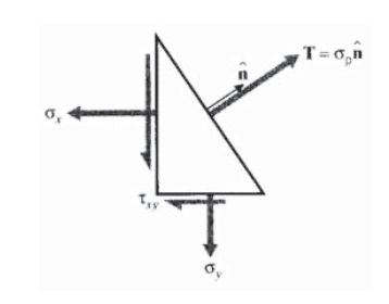
The Mohr’s circle procedure is not capable of finding principal stresses for three-dimensional stress states, and a more general method is needed. In three dimensions, we seek orientations of axes such that no shear stresses appear, leaving only normal stresses in three orthogonal directions. The vanishing of shear stresses on a plane means that the stress vector \(T\) is normal to the plane, illustrated in two dimensions in Figure 11. The traction vector can therefore be written as
\[T= \sigma_p \hat{n}\nonumber\]
where \(\sigma_p\) is a simple scalar quantity, the magnitude of the stress vector. Using this in Cauchy’s relation:
\[\sigma \hat{n} = T = \sigma_p \hat{n}\nonumber\]
\[(\sigma - \sigma_p I) \hat{n} = 0\]
Here \(I\) is the unit matrix. This system will have a nontrivial solution (\(\hat{n} \ne 0\)) only if its determinant is zero:
\[|\sigma - \sigma_p I| = \left | \begin{matrix} \sigma_x - \sigma_p & \tau_{xy} & \tau_{xz} \\ \tau_{xy} & \sigma_y - \sigma_p & \tau_{yz} \\ \tau_{xz} & \tau_{yz} & \sigma_z - \sigma_p \end{matrix} \right | = 0\nonumber\]
Expanding the determinant yields a cubic polynomial equation in \(\sigma_p\):
\[f(\sigma_p) = \sigma_p^3 - I_1 \sigma_p^3 + I_2 \sigma_p - I_3 = 0\]
This is the characteristic equation for stress, where the coefficients are
\[I_1 = \sigma_x + \sigma_y + \sigma_z = \sigma_{kk}\]
\[I_2 = \sigma_x \sigma_y + \sigma_x \sigma_z + \sigma_y \sigma_z - \tau_{xy}^2 - \tau_{yz}^2 - \tau_{xz}^2 = \dfrac{1}{2} (\sigma_{ii} \sigma_{jj} - \sigma_{ij} \sigma_{ij})\]
\[I_3 = \text{det} |\sigma| = \dfrac{1}{3} \sigma_{ij} \sigma_{jk} \sigma_{ki}\]
These \(I\) parameters are known as the invariants of the stress state; they do not change with transformation of the coordinates and can be used to characterize the overall nature of the stress. For instance \(I_1\), which has been identified earlier as the trace of the stress matrix, will be seen in a later section to be a measure of the tendency of the stress state to induce hydrostatic dilation or compression. We have already noted that the stress state is one of pure shear if its trace vanishes.
Since the characteristic equation is cubic in \(\sigma_p\), it will have three roots, and it can be shown that all three roots must be real. These roots are just the principal stresses \(\sigma_{p1}\), \(\sigma_{p2}\) and \(\sigma_{p3}\).
Example \(\PageIndex{6}\)
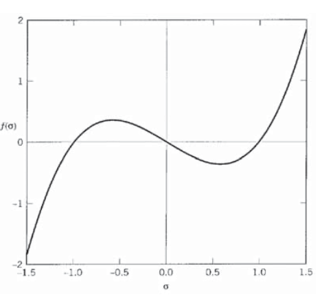
Consider a state of simple shear with \(\tau_{xy} = 1\) and all other stresses zero:
\[|\sigma| = \begin{bmatrix} 0 & 1 & 0 \\ 1 & 0 & 0 \\ 0 & 0 & 0 \end{bmatrix}\nonumber\]
The invariants are
\[I_1 = 0, I_2 = -1, I_3 = 0\nonumber\]
and the characteristic equation is
\[\sigma_p^3 - \sigma_p = 0\nonumber\]
This equation has roots of (-1, 0, 1) corresponding to principal stresses \(\sigma_{p1} = 1, \sigma_{p2} = 0, \sigma_{p3} = -1\), and is plotted in Figure 12. This is the same stress state considered in Example 4, and the roots of the characteristic equation agree with the principal values shown by the Mohr’s circle.
Exercise \(\PageIndex{1}\)
Develop an expression for the stress needed to cause transverse failure in a unidirectionally oriented composite as a function of the angle between the load direction and the fiber direction, and show this function in a plot of strength versus \(\theta\).
Exercise \(\PageIndex{2}\)
Use a free-body force balance to derive the two-dimensional Cartesian stress transformation equations as
\[\begin{array} {rcl} {\sigma_{x'}} & = & {\sigma_x \cos^2 \theta + \sigma_y \sin^2 \theta + 2 \tau_{xy} \sin \theta \cos \theta} \\ {\sigma_{y'}} & = & {\sigma_x \sin^2 \theta + \sigma_y \cos^2 \theta - 2 \tau_{xy} \sin \theta \cos \theta} \\ {\tau_{x'y'}} & = & {(\sigma_y - \sigma_x) \sin \theta \cos \theta + \tau_{xy} (\cos^2 \theta - \sin^2 \theta)} \end{array} \nonumber\]
Or
\[\left \{\begin{array} {c} {\sigma_{x'}} \\ {\sigma_{y'}} \\ {\tau_{x'y'}} \end{array} \right \} = \begin{bmatrix} c^2 & s^2 & 2sc \\ s^2 & c^2 & -2sc \\ -sc & sc & c^2 - s^2 \end{bmatrix} \left \{\begin{array} {c} {\sigma_{x}} \\ {\sigma_{y}} \\ {\tau_{xy}} \end{array} \right \}\nonumber\]
where \(c = \cos \theta\) and \(s = \sin \theta\)
Exercise \(\PageIndex{3}\)
Develop mathematical relations for displacements and gradients along transformed axes of the form
\[u' = u \cos \theta + v \sin \theta \nonumber\]
\[\dfrac{\partial}{\partial x'} = \dfrac{\partial}{\partial x} \cdot \dfrac{\partial x}{\partial x'} + \dfrac{\partial}{\partial y} \cdot \dfrac{\partial y}{\partial x'} = \dfrac{\partial}{\partial x} \cdot \cos \theta + \dfrac{\partial}{\partial y} \cdot \sin \theta \nonumber\]
with analogous expressions for \(v'\) and \(\partial /\partial y'\). Use these to obtain the strain transformation equations (Equation 3.3.6).
Exercise \(\PageIndex{4}\)
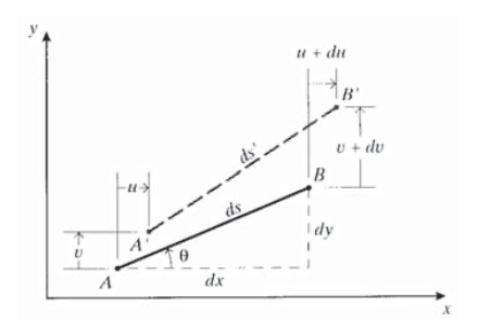
Consider a line segment \(AB\) of length \(ds^2 = dx^2 + dy^2\), oriented at an angle \(\theta\) from the Cartesian \(x - y\) axes as shown. Let the differential displacement of end \(B\) relative to end \(A\) be
\[du = \dfrac{\partial u}{\partial x} dx + \dfrac{\partial u}{\partial y} dy\nonumber\]
\[dv = \dfrac{\partial v}{\partial x} dx + \dfrac{\partial v}{\partial y} dy\nonumber\]
Use this geometry to derive the strain transformation equations (Equation 3.3.6), where the \(x'\) axis is along line \(AB\).
Exercise \(\PageIndex{5}\)
Employ double-angle trigonometric relations to show that the two-dimensional Cartesian stress transformation equations can be written in the form
\[\begin{array} {rcr} {\sigma_{x'}} & = & {\tfrac{\sigma_x + \sigma_y}{2} + \tfrac{\sigma_x - \sigma_y}{2} \cos 2 \theta + \tau_{xy} \sin 2 \theta} \\ {\tau_{x'y'}} & = & {-\tfrac{\sigma_x - \sigma_y}{2} \sin 2 \theta + \tau_{xy} \cos 2\theta} \\ {\sigma_{y'}} & = & {\tfrac{\sigma_x + \sigma_y}{2} + \tfrac{\sigma_x - \sigma_y}{2} \cos 2 \theta - \tau_{xy} \sin 2 \theta} \end{array} \nonumber\]
Use these relations to justify the Mohr’s circle construction.
Exercise \(\PageIndex{6}\)
Use matrix multiplication (Eqns. 3.3.5 or 3.3.8) to transform the following stress and strain states to axes rotated by \(\theta = 30^{\circ}\) from the original \(x-y\) axes.
(a)
\[\sigma = \left \{ \begin{array} {c} {1.0} \\ {-2.0} \\ {3.0} \end{array} \right \}\nonumber\]
(b)
\[\epsilon = \left \{ \begin{array} {c} {0.01} \\ {-0.02} \\ {0.03} \end{array} \right \}\nonumber\]
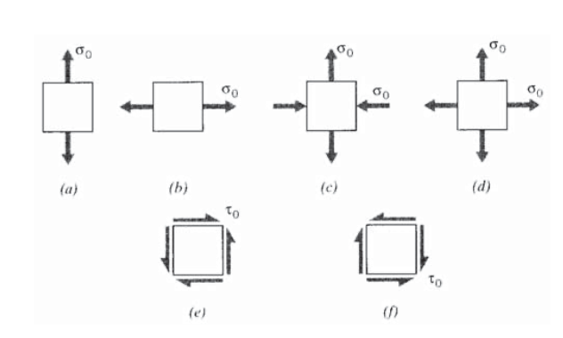
Exercise \(\PageIndex{7}\)
Sketch the Mohr’s circles for each of the stress states shown in the figure below.
Exercise \(\PageIndex{8}\)
Construct Mohr’s circle solutions for the transformations of Exercise \(\PageIndex{6}\).
Exercise \(\PageIndex{9}\)
Draw the Mohr’s circles and determine the magnitudes of the principal stresses for the following stress states. Denote the principal stress state on a suitably rotated stress square.
(a) \(\sigma_x = 30\) MPa, \(\sigma_y = -10\) MPa, \(\tau_{xy} = 25\) MPa.
(b) \(\sigma_x = -30\) MPa, \(\sigma_y = -90\) MPa, \(\tau_{xy} = -40\) MPa.
(c) \(\sigma_x = -10\) MPa, \(\sigma_y = 20\) MPa, \(\tau_{xy} = -15\) MPa.
Exercise \(\PageIndex{10}\)
Show that the values of principal stresses given by Mohr’s circle agree with those obtained mathematically by setting to zero the derivatives of the stress with respect to the transformation angle.
Exercise \(\PageIndex{11}\)
For the 3-dimensional stress state \(\sigma_x = 25, \sigma_y = -15, \sigma_z = -30, \tau_{yz} = 20, \tau_{xz} = 10, \tau_{xy} = 30\) (all in MPa):
(a)Determine the stress state for Euler angles \(\psi = 20^{\circ}\), \(\theta = 30^{\circ}\), \(\phi = 25^{\circ}\).
(b) Plot the characteristic equation.
(c) Determine the principal stresses.