3.4: Constitutive Relations

Introduction

The modules on kinematics (Module 8), equilibrium (Module 9), and tensor transformations (Module 10) contain concepts vital to Mechanics of Materials, but they do not provide insight on the role of the material itself. The kinematic equations relate strains to displacement gradients, and the equilibrium equations relate stress to the applied tractions on loaded boundaries and also govern the relations among stress gradients within the material. In three dimensions there are six kinematic equations and three equilibrum equations, for a total of nine. However, there are fifteen variables: three displacements, six strains, and six stresses. We need six more equations, and these are provided by the material’s consitutive relations: six expressions relating the stresses to the strains. These are a sort of mechanical equation of state, and describe how the material is constituted mechanically.

With these constitutive relations, the vital role of the material is reasserted: The elastic constants that appear in this module are material properties, subject to control by processing and microstructural modification as outlined in Module 2. This is an important tool for the engineer, and points up the necessity of considering design of the material as well as with the material.

Isotropic elastic materials

In the general case of a linear relation between components of the strain and stress tensors, we might propose a statement of the form

\[\epsilon_{ij} = S_{ijkl} \sigma_{kl}\nonumber\]

where the \(S_{ijkl}\) is a fourth-rank tensor. This constitutes a sequence of nine equations, since each component of \(\epsilon_{ij}\) is a linear combination of all the components of \(\sigma_{ij}\). For instance:

\[\epsilon_{23} = S_{2311} \sigma_{11} + S_{2312} \sigma_{12} + \cdots + S_{2333} \epsilon_{33}\nonumber\]

Based on each of the indices of \(S_{ijkl}\) taking on values from 1 to 3, we might expect a total of 81 independent components in \(S\). However, both \(\epsilon_{ij}\) and \(\sigma_{ij}\) are symmetric, with six rather than nine independent components each. This reduces the number of \(S\) components to 36, as can be seen from a linear relation between the pseudovector forms of the strain and stress:

\[\left \{ \begin{matrix} \epsilon_x \\ \epsilon_y \\ \epsilon_z \\ \gamma_{yz} \\ \gamma_{xz} \\ \gamma_{xy} \end{matrix} \right \} = \begin{bmatrix} S_{11} & S_{12} & \cdots & S_{16} \\ S_{21} & S_{22} & \cdots & S_{26} \\ \cdots & \cdots & \cdots & \cdots \\ S_{61} & S_{62} & \cdots & S_{66} \end{bmatrix} \left \{ \begin{matrix} \sigma_x \\ \sigma_y \\ \sigma_z \\ \tau_{yz} \\ \tau_{xz} \\ \tau_{xy} \end{matrix} \right \}\]

It can be shown(G.M. Mase, Schaum’s Outline of Theory and Problems of Continuum Mechanics, McGraw-Hill, 1970.) that the \(S\) matrix in this form is also symmetric. It therefore it contains only 21 independent elements, as can be seen by counting the elements in the upper right triangle of the matrix, including the diagonal elements (1 + 2 + 3 + 4 + 5 + 6 = 21).

If the material exhibits symmetry in its elastic response, the number of independent elements in the \(S\) matrix can be reduced still further. In the simplest case of an isotropic material, whose stiffnesses are the same in all directions, only two elements are independent. We have earlier shown that in two dimensions the relations between strains and stresses in isotropic materials can be written as

\[\begin{array} {c} {\epsilon_x = \dfrac{1}{E} (\sigma_x - \nu \sigma_y)} \\ {\epsilon_y = \dfrac{1}{E} (\sigma_y - \nu \sigma_x)} \\ {\gamma_{xy} = \dfrac{1}{G} \tau_{xy}} \end{array}\]

along with the relation

\[G = \dfrac{E}{2(1 + \nu)}\nonumber\]

Extending this to three dimensions, the pseudovector-matrix form of Equation 3.4.1 for isotropic mate- rials is

\[\left \{ \begin{matrix} \epsilon_x \\ \epsilon_y \\ \epsilon_z \\ \gamma_{yz} \\ \gamma_{xz} \\ \gamma_{xy} \end{matrix} \right \} = \begin{bmatrix} \tfrac{1}{E} & \tfrac{-\nu}{E} & \tfrac{-\nu}{E} & 0 & 0 & 0 \\ \tfrac{-\nu}{E} & \tfrac{1}{E} & \tfrac{-\nu}{E} & 0 & 0 & 0 \\ \tfrac{-\nu}{E} & \tfrac{-\nu}{E} & \tfrac{1}{E} & 0 & 0 & 0 \\ 0 & 0 & 0 & \tfrac{1}{G} & 0 & 0 \\ 0 & 0 & 0 & 0 & \tfrac{1}{G} & 0 \\ 0 & 0 & 0 & 0& 0 & \tfrac{1}{G} \end{bmatrix} \left \{ \begin{matrix} \sigma_x \\ \sigma_y \\ \sigma_z \\ \tau_{yz} \\ \tau_{xz} \\ \tau_{xy} \end{matrix} \right \}\]

The quantity in brackets is called the compliance matrix of the material, denoted \(S\) or \(S_{ij}\). It is important to grasp the physical significance of its various terms. Directly from the rules of matrix multiplication, the element in the \(i^{th}\) row and \(j^{th}\) column of \(S_{ij}\) is the contribution of the \(j^{th}\) stress to the \(i^{th}\) strain. For instance the component in the 1,2 position is the contribution of the \(y\)-direction stress to the \(x\)-direction strain: multiplying \(\sigma_y\) by \(1/E\) gives the \(y\)-direction strain generated by \(\sigma_y\), and then multiplying this by \(-\nu\) gives the Poisson strain induced in the \(x\) direction. The zero elements show the lack of coupling between the normal and shearing components.

The isotropic constitutive law can also be written using index notation as (see Exercise \(\PageIndex{1}\))

\[\epsilon_{ij} = \dfrac{1 + \nu}{E} \sigma_{ij} - \dfrac{\nu}{E} \delta_{ij} \sigma_{kk}\]

where here the indicial form of strain is used and \(G\) has been eliminated using \(G = E/2(1 + \nu)\) The symbol \(\delta_{ij}\) is the Kroenecker delta, described in the Module on Matrix and Index Notation.

If we wish to write the stresses in terms of the strains, Eqn 3.4.3 can be inverted. In cases of plane stress (\(\sigma_z = \tau_{xz} = \tau_{yz} = 0\)), this yields

\[\left \{ \begin{matrix} \sigma_x \\ \sigma_y \\ \tau_{xy} \end{matrix} \right \} = \dfrac{E}{1-\nu^2} \begin{bmatrix} 1 & \nu & 0 \\ \nu & 1 & 0 \\ 0 & 0 & (1 - \nu)/2 \end{bmatrix} \left \{ \begin{matrix} \epsilon_x \\ \epsilon_y \\ \gamma_{xy} \end{matrix} \right \}\]

where again \(G\) has been replaced by \(E/2(1 + \nu)\). Or, in abbreviated notation:

\[\sigma = D \epsilon\]

where \(D = S^{-1}\) is the stiffness matrix.

Hydrostatic and distortional components

Figure 1: Hydrostatic compression.

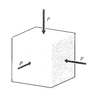
A state of hydrostatic compression, depicted in Figure 1, is one in which no shear stresses exist and where all the normal stresses are equal to the hydrostatic pressure:

\[\sigma_x = \sigma_y = \sigma_z = -p\nonumber\]

where the minus sign indicates that compression is conventionally positive for pressure but negative for stress. For this stress state it is obviously true that

\[\dfrac{1}{3} (\sigma_x + \sigma_y + \sigma_z) = \dfrac{1}{3} \sigma_{kk} = -p\nonumber\]

so that the hydrostatic pressure is the negative mean normal stress. This quantity is just one third of the stress invariant \(I_1\), which is a reflection of hydrostatic pressure being the same in all directions, not varying with axis rotations.

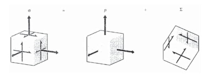
In many cases other than direct hydrostatic compression, it is still convenient to "dissociate" the hydrostatic (or "dilatational") component from the stress tensor:

\[\sigma_{ij} = \dfrac{1}{3} \sigma_{kk} \delta_{ij} + \sum_{ij}\]

Here \(\sum_{ij}\) is what is left over from \(\sigma_{ij}\) after the hydrostatic component is subtracted. The \(\sum_{ij}\) tensor can be shown to represent a state of pure shear, i.e. there exists an axis transformation such that all normal stresses vanish (see Exercise \(\PageIndex{5}\)). The \(\sum_{ij}\) is called the distortional, or deviatoric, component of the stress. Hence all stress states can be thought of as having two components as shown in Figure 2, one purely extensional and one purely distortional. This concept is convenient because the material responds to these stress components is very different ways. For instance, plastic and viscous flow is driven dominantly by distortional components, with the hydrostatic component causing only elastic deformation.

Figure 2: Dilatational and deviatoric components of the stress tensor.

Example \(\PageIndex{1}\)

Consider the stress state

\[\sigma = \begin{bmatrix} 5 & 6 & 7 \\ 6 & 8 & 9 \\ 7 & 9 & 2 \end{bmatrix}, \text{ GPa} \nonumber\]

The mean normal stress is \(\sigma_{kk}/3 = (5 + 8 + 2)/3 = 5\), so the stress decomposition is

\[\sigma = \dfrac{1}{3} \sigma_{kk} \delta_{ij} + \sum_{ij} = \begin{bmatrix} 5 & 0 & 0 \\ 0 & 5 & 0 \\ 0 & 0 & 5 \end{bmatrix} + \begin{bmatrix} 0 & 6 & 7 \\ 6 & 3 & 9 \\ 7 & 9 & -3 \end{bmatrix}\nonumber\]

It is not obvious that the deviatoric component given in the second matrix represents pure shear, since there are nonzero components on its diagonal. However, a stress transformation using Euler angles \(\psi = \phi = 0, \theta = -9.22^{\circ}\) gives the stress state

\[\sum' = \begin{bmatrix} 0.00 & 4.80 & 7.87 \\ 4.80 & 0.00 & 9.49 \\ 7.87 & 9.49 & 0.00 \end{bmatrix}\nonumber\]

The hydrostatic component of stress is related to the volumetric strain through the modulus of compressibility (\(-p = K \Delta V/V\)), so

\[\dfrac{1}{3} \sigma_{kk} = K\epsilon_{kk}\]

Similarly to the stress, the strain can also be dissociated as

\[\epsilon_{ij} = \dfrac{1}{3} \epsilon_{kk} \delta_{ij} + e_{ij}\nonumber\]

where \(e_{ij}\) is the deviatoric component of strain. The deviatoric components of stress and strain are related by the material’s shear modulus:

\[\sum_{ij} = 2Ge_{ij}\]

where the factor 2 is needed because tensor descriptions of strain are half the classical strains for which values of \(G\) have been tabulated. Writing the constitutive equations in the form of Eqns. 3.4.8 and 3.4.9 produces a simple form without the coupling terms in the conventional \(E-\nu\) form.

Example \(\PageIndex{2}\)

Using the stress state of the previous example along with the elastic constants for steel (\(E = 207\) GPa, \(\nu = 0.3\), \(K = E/3(1 - 2\nu) = 173\) GPa, \(G = E/2(1 + \nu) = 79.6\) GPa), the dilatational and distortional components of strain are

\[\delta_{ij} \epsilon_{kk} = \dfrac{\delta_{ij} \sigma_kk}{3K} = \begin{bmatrix} 0.0289 & 0 & 0 \\ 0 & 0.0289 & 0 \\ 0 & 0 & 0.0289 \end{bmatrix}\nonumber\]

\[e_{ij} = \dfrac{\sum_{ij}}{2G} = \begin{bmatrix} 0 & 0.0378 & 0.0441 \\ 0.0378 & 0.0189 & 0.0567 \\ 0.0441 & 0.0567 & -0.0189 \end{bmatrix}\nonumber\]

The total strain is then

\[\epsilon_{ij} = \dfrac{1}{3} \epsilon_{kk} \delta_{ij} + e_{ij} = \begin{bmatrix} 0.00960 & 0.0378 & 0.0441 \\ 0.0378 & 0.0285 & 0.0567 \\ 0.0441 & 0.0567 & -0.00930 \end{bmatrix}\nonumber\]

If we evaluate the total strain using Equation 3.4.4, we have

\(\epsilon_{ij} = \dfrac{1 + \nu}{E} \sigma_ij - \dfrac{\nu}{E} \delta_{ij} \sigma_{kk} = \begin{bmatrix} 0.00965 & 0.0377 & 0.0440 \\ 0.0377 & 0.0285 & 0.0565 \\ 0.0440 & 0.0565 & -0.00915 \end{bmatrix}\nonumber\]

These results are the same, differing only by roundoff error.

Finite strain model

When deformations become large, geometrical as well as material nonlinearities can arise that are important in many practical problems. In these cases the analyst must employ not only a different strain measure, such as the Lagrangian strain described in Module 8, but also different stress measures (the "Second Piola-Kirchoff stress" replaces the Cauchy stress when Lagrangian strain is used) and different stress-strain constitutive laws as well. A treatment of these formulations is beyond the scope of these modules, but a simple nonlinear stress-strain model for rubbery materials will be outlined here to illustrate some aspects of finite strain analysis. The text by Bathe(K.-J. Bathe, Finite Element Procedures in Engineering Analysis, Prentice-Hall, 1982.) provides a more extensive discussion of this area, including finite element implementations.

In the case of small displacements, the strain \(\epsilon_x\) is given by the expression:

\[\epsilon_x = \dfrac{1}{E} [\sigma_x - \nu (\sigma_y + \sigma_z)]\nonumber\]

For the case of elastomers with \(\nu = 0.5\), this can be rewritten in terms of the mean stress \(\sigma_m = (\sigma_x + \sigma_y + \sigma_z)/3\) as:

\[2 \epsilon_x = \dfrac{3}{E} (\sigma_x - \sigma_m)\nonumber\]

For the large-strain case, the following analogous stress-strain relation has been proposed:

\[\lambda_x^2 = 1 + 2 \epsilon_x = \dfrac{3}{E} (\sigma_x - \sigma_m^*)\]

where here \(\epsilon_x\) is the Lagrangian strain and \(\sigma_m^*\) is a parameter not necessarily equal to \(\sigma_m\). The \(\sigma_m^*\) parameter can be found for the case of uniaxial tension by considering the transverse contractions \(\lambda_y = \lambda_z\):

\[\lambda_y^2 = \dfrac{3}{E} (\sigma_y - \sigma_m^*)\nonumber\]

Since for rubber \(\lambda_x \lambda_y \lambda_z = 1\), \(\lambda_y^2 = 1/\lambda_x\). Making this substitution and solving for \(\sigma_m^*\):

\[\sigma_m^* = \dfrac{-E\lambda_y^2}{3} = \dfrac{-E}{3\lambda_x}\nonumber\]

Substituting this back into Equation 3.4.10,

\[\lambda_x^2 = \dfrac{E}{3} (\sigma_x - \dfrac{E}{3\lambda_x})\nonumber\]

Solving for \(\sigma_x\),

\[\sigma_x = \dfrac{E}{3} (\lambda_x^2 - \dfrac{1}{\lambda_x})\nonumber\]

Here the stress \(\sigma_x = F/A\) is the "true" stress based on the actual (contracted) cross-sectional area. The "engineering" stress \(\sigma_e = F/A_0\) based on the original area \(A_0 = A \lambda_x\) is:

\[\sigma_e = \dfrac{\sigma_x}{\lambda_x} = G\left (\lambda_x - \dfrac{1}{\lambda_x^2} \right )\nonumber\]

where \(G = E/2(1 + \nu) = E/3\) for \(\nu = 1/2\). This result is the same as that obtained in Module 2 by considering the force arising from the reduced entropy as molecular segments spanning crosslink sites are extended. It appears here from a simple hypothesis of stress-strain response, using a suitable measure of finite strain.

Anisotropic materials

Figure 3: An orthotropic material.

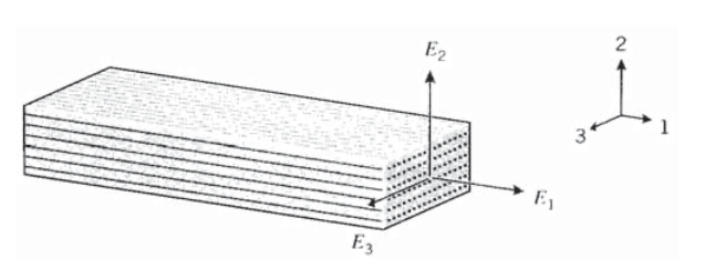
If the material has a texture like wood or unidirectionally-reinforced fiber composites as shown in Figure 3, the modulus \(E_1\) in the fiber direction will typically be larger than those in the transverse directions (\(E_2\) and \(E_3\)). When \(E_1 \ne E_2 \ne E_3\), the material is said to be orthotropic. It is common, however, for the properties in the plane transverse to the fiber direction to be isotropic to a good approximation \((E_2 = E_3)\); such a material is called transversely isotropic. The elastic constitutive laws must be modified to account for this anisotropy, and the following form is an extension of Equation 3.4.3 for transversely isotropic materials:

\[\left \{ \begin{matrix} \epsilon_1 & \epsilon_2 & \gamma_{12} \end{matrix} \right \} = \begin{bmatrix} 1/E_1 & -\nu_{21}/E_2 & 0 \\ -\nu_{12}/E_1 & 1/E_2 & 0 \\ 0 & 0 & 1/G_{12} \end{bmatrix} \left \{ \begin{matrix} \sigma_1 & \sigma_2 & \tau_{12} \end{matrix} \right \}\]

The parameter \(\nu_{12}\) is the principal Poisson’s ratio; it is the ratio of the strain induced in the 2-direction by a strain applied in the 1-direction. This parameter is not limited to values less than 0.5 as in isotropic materials. Conversely, \(\nu_{21}\) gives the strain induced in the 1-direction by a strain applied in the 2-direction. Since the 2-direction (transverse to the fibers) usually has much less stiffness than the 1-direction, it should be clear that a given strain in the 1-direction will usually develop a much larger strain in the 2-direction than will the same strain in the 2-direction induce a strain in the 1-direction. Hence we will usually have \(\nu_{12} > \nu_{21}\). There are five constants in the above equation (\(E_1, E_2, \nu_{12}, \nu_{21}\) and \(G_{12}\)). However, only four of them are independent; since the \(S\) matrix is symmetric, \(\nu_{21}/E2 = \nu_{12}/E1\).

A table of elastic constants and other properties for widely used anisotropic materials can be found in the Module on Composite Ply Properties.

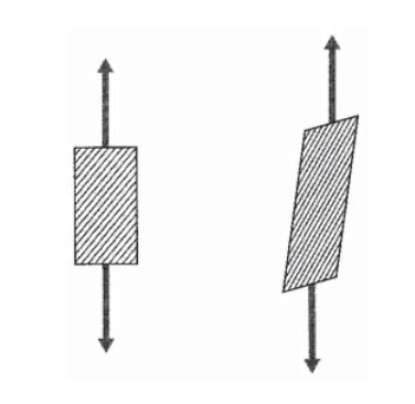
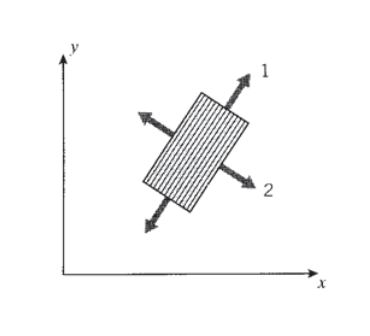
The simple form of Equation 3.4.11, with zeroes in the terms representing coupling between normal and shearing components, is obtained only when the axes are aligned along the principal material directions; i.e. along and transverse to the fiber axes. If the axes are oriented along some other direction, all terms of the compliance matrix will be populated, and the symmetry of the material will not be evident. If for instance the fiber direction is off-axis from the loading direction, the material will develop shear strain as the fibers try to orient along the loading direction as shown in Figure 4. There will therefore be a coupling between a normal stress and a shearing strain, which never occurs in an isotropic material.

Figure 4: Shear-normal coupling.

The transformation law for compliance can be developed from the transformation laws for strains and stresses, using the procedures described in Module 10 (Transformations). By successive transformations, the pseudovector form for strain in an arbitrary \(x-y\) direction shown in Figure 5 is related to strain in the 1-2 (principal material) directions, then to the stresses in the 1-2 directions, and finally to the stresses in the \(x-y\) directions. The final grouping of transformation matrices relating the \(x-y\) strains to the \(x-y\) stresses is then the transformed compliance matrix in the \(x-y\) direction:

Figure 5: Axis transformation for constitutive equations.

\[\left \{ \begin{matrix} \epsilon_x & \epsilon_y & \gamma_{xy} \end{matrix} \right \} = R \left \{ \begin{matrix} \epsilon_x & \epsilon_y & \tfrac{1}{2} \gamma_{xy} \end{matrix} \right \} = RA^{-1} \left \{ \begin{matrix} \epsilon_1 & \epsilon_2 & \tfrac{1}{2} \gamma_{12} \end{matrix} \right \} = RA^{-1}R^{-1} \left \{ \begin{matrix} \epsilon_1 & \epsilon_2 & \gamma_{12} \end{matrix} \right \}\nonumber\]

\[=RA^{-1}R^{-1} S \left \{ \begin{matrix} \sigma_1 & \sigma_2 & \tau_{12} \end{matrix} \right \} = RA^{-1}RSA \left \{ \begin{matrix} \sigma_x & \sigma_y & \sigma_{xy} \end{matrix} \right \} = \bar{S} \left \{ \begin{matrix} \sigma_x & \sigma_y & \sigma_{xy} \end{matrix} \right \}\nonumber\]

where \(\bar{S}\) is the transformed compliance matrix relative to \(x-y\) axes. Here \(A\) is the transformation matrix, and \(R\) is the Reuter’s matrix defined in the Module on Tensor Transformations. The inverse of \(\bar{S}\) is \(\bar{D}\), the stiffness matrix relative to \(x-y\) axes:

\[\bar{S} = RA^{-1}SA, \ \ \bar{D} = \bar{S}^{-1}\]

Example \(\PageIndex{1}\)

Consider a ply of Kevlar-epoxy composite with a stiffnesses \(E_1 = 82, E_2 = 4, G_{12} = 2.8\) (all GPa) and \(\nu_{12} = 0.25\). The compliance matrix \(S\) in the 1-2 (material) direction is:

\[S = \begin{bmatrix} 1/E_1 & -\nu_{21} /E_2 & 0 \\ -\nu_{12} /E_1 & 1/E_2 & 0 \\ 0 & 0 & 1/G_{12} \end{bmatrix} = \begin{bmatrix} .1220 \times 10^{-10} & -.3050 \times 10^{-11} & 0 \\ -.3050 \times 10^{-11} & .2500 \times 10^{-9} & 0 \\ 0 & 0 & .3571 \times 10^{-9} \end{bmatrix}\nonumber\]

If the ply is oriented with the fiber direction (the "1" direction) at \(\theta = 30^{\circ}\) from the \(x-y\) axes, the appropriate transformation matrix is

\[A = \begin{bmatrix} c^2 & s^2 & 2sc \\ s^2 & c^2 & -2sc \\ -sc & sc & c^2 - s^2 \end{bmatrix} = \begin{bmatrix} .7500 & .2500 & .8660 \\ .2500 & .7500 & -.8600 \\ -.4330 & .4330 & .5000 \end{bmatrix}\nonumber\]

The compliance matrix relative to the \(x-y\) axes is then

\[\bar{S} = RA^{-1}R^{-1}SA = \begin{bmatrix} .8830 \times 10^{-10} & -.1970 \times 10^{-10} & -1.222 \times 10^{-9} \\ -.1971 \times 10^{-10} & .2072 \times 10^{-9} & -.8371 \times 10^{-10} \\ 1.222 \times 10^{-9} & -.8369 \times 10^{-10} & -2905 \times 10^{-9} \end{bmatrix}\nonumber\]

Note that this matrix is symmetric (to within numerical roundoff error), but that nonzero coupling values exist. A user not aware of the internal composition of the material would consider it completely anisotropic.

The apparent engineering constants that would be observed if the ply were tested in the \(x-y\) rather than 1-2 directions can be found directly from the trasnformed \(\bar{S}\) matrix. For instance, the apparent elastic modulus in the \(x\) direction is \(E_x = 1/\bar{S}_{1,1} = 1/(.8830 \times 10^{-10} = 11.33\) GPa.

Exercise \(\PageIndex{1}\)

Expand the indicial forms of the governing equations for solid elasticity in three dimensions:

\[\text{equilibrium: } \sigma_{ij,j} = 0\nonumber\]

\[\text{kinematric: } \epsilon_{ij} = (u_{i,j} + u_{j, i})/2\nonumber\]

\[\text{constitutive: } \epsilon_{ij} = \dfrac{1 + \nu}{E} \sigma_{ij} - \dfrac{\nu}{E} \delta_{ij} \sigma_{kk} + \alpha \delta_{ij} \Delta T\nonumber\]

where \(\alpha\) is the coefficient of linear thermal expansion and \(\Delta T\) is a temperature change.

Exercise \(\PageIndex{2}\)

(a) Write out the compliance matrix \(S\) of Equation 3.4.3 for polycarbonate using data in the Module on Material Properties.

(b) Use matrix inversion to obtain the stiffness matrix \(D\).

(c) Use matrix multiplication to obtain the stresses needed to induce the strains

\[\epsilon = \left \{ \begin{matrix} \epsilon_x \\ \epsilon_y \\ \epsilon_z \\ \gamma_{yz} \\ \gamma_{xz} \\ \gamma_{xy} \end{matrix} \right \} = \left \{ \begin{matrix} 0.02 \\ 0.0 \\ 0.03 \\ 0.01 \\ 0.025 \\ 0.0 \end{matrix} \right \}\nonumber\]

Exercise \(\PageIndex{3}\)

(a) Write out the compliance matrix \(S\) of Equation 3.4.3 for an aluminum alloy using data in the Module on Material Properties.

(b) Use matrix inversion to obtan the stiffness matrix \(D\).

(c) Use matrix multiplication to obtain the stresses needed to induce the strains

\[\epsilon = \left \{ \begin{matrix} \epsilon_x \\ \epsilon_y \\ \epsilon_z \\ \gamma_{yz} \\ \gamma_{xz} \\ \gamma_{xy} \end{matrix} \right \} = \left \{ \begin{matrix} 0.01 \\ 0.02 \\ 0.0 \\ 0.0 \\ 0.15 \\ 0.0 \end{matrix} \right \}\nonumber\]

Exercise \(\PageIndex{4}\)

Given the stress tensor

\[\sigma_{ij} = \begin{bmatrix} 1 & 2 & 3 \\ 2 & 4 & 5 \\ 3 & 5 & 7 \end{bmatrix} \ \ \text{(MPa)}\nonumber\]

(a) Dissociate \(\sigma_{ij}\) into deviatoric and dilatational parts \(\sum_{ij}\) and \((1/3) \sigma_{kk} \delta_{ij}\).

(b) Given \(G = 357\) MPa and \(K = 1.67\) GPa, obtain the deviatoric and dilatational strain tensors \(e_{ij}\) and \((1/3)\epsilon_{kk} \delta_{ij}\).

(c) Add the deviatoric and dilatational strain components obtained above to obtain the total strain tensor \(\epsilon_{ij}\).

(d) Compute the strain tensor \(\epsilon_{ij}\) using the alternate form of the elastic constitutive law for isotropic elastic solids:

\[\epsilon_{ij} = \dfrac{1 + \nu}{E} \sigma_{ij} - \dfrac{\nu}{E} \delta_{ij} \sigma_{kk}\nonumber\]

Compare the result with that obtained in (c).

Exercise \(\PageIndex{5}\)

Provide an argument that any stress matrix having a zero trace can be transformed to one having only zeroes on its diagonal; i.e. the deviatoric stress tensor \(\sum_{ij}\) represents a state of pure shear.

Exercise \(\PageIndex{6}\)

Write out the \(x-y\) two-dimensional compliance matrix \(\bar{S}\) and stiffness matrix \(\bar{D}\) (Equation 3.4.12) for a single ply of graphite/epoxy composite with its fibers aligned along the \(x\) axes.

Exercise \(\PageIndex{7}\)

Write out the \(x-y\) two-dimensional compliance matrix \(\bar{S}\) and stiffness matrix \(\bar{D}\) (Equation 3.4.12) for a single ply of graphite/epoxy composite with its fibers aligned 30\(^{\circ}\) from the \(x\) axis.