4.1: Shear and Bending Moment Diagrams
- Page ID
- 44540

Introduction
Beams are long and slender structural elements, differing from truss elements in that they are called on to support transverse as well as axial loads. Their attachment points can also be more complicated than those of truss elements: they may be bolted or welded together, so the attachments can transmit bending moments or transverse forces into the beam. Beams are among the most common of all structural elements, being the supporting frames of airplanes, buildings, cars, people, and much else.
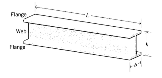
The nomenclature of beams is rather standard: as shown in Figure 1, \(L\) is the length, or span; \(b\) is the width, and \(h\) is the height (also called the depth). The cross-sectional shape need not be rectangular, and often consists of a vertical web separating horizontal fllanges at the top and bottom of the beam (There is a standardized protocol for denoting structural steel beams; for instance W 8 × 40 indicates a wide-ffllange beam with a nominal depth of 8′′ and weighing 40 lb/ft of length)
As will be seen in Modules 13 and 14, the stresses and deflections induced in a beam under bending loads vary along the beam's length and height. The first step in calculating these quantities and their spatial variation consists of constructing shear and bending moment diagrams, \(V(x)\) and \(M(x)\), which are the internal shearing forces and bending moments induced in the beam, plotted along the beam's length. The following sections will describe how these diagrams are made.
Free-body diagrams
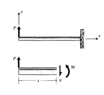
As a simple starting example, consider a beam clamped (\cantilevered") at one end and subjected to a load \(P\) at the free end as shown in Figure 2. A free body diagram of a section cut transversely at position \(x\) shows that a shear force \(V\) and a moment \(M\) must exist on the cut section to maintain equilibrium. We will show in Module 13 that these are the resultants of shear and normal stresses that are set up on internal planes by the bending loads. As usual, we will consider section areas whose normals point in the +\(x\) direction to be positive; then shear forces pointing in the +\(y\) direction on +\(x\) faces will be considered positive. Moments whose vector direction as given by the right-hand rule are in the +\(z\) direction (vector out of the plane of the paper, or tending to cause counterclockwise rotation in the plane of the paper) will be positive when acting on +\(x\) faces. Another way to recognize positive bending moments is that they cause the bending shape to be concave upward. For this example beam, the statics equations give:
\[\sum F_y = 0 = V + P \Rightarrow V = \text{constant} = -P\]
\[\sum M_0 = 0 = -M + Px \Rightarrow M = M(x) = Px\]
Note that the moment increases with distance from the loaded end, so the magnitude of the maximum value of \(M\) compared with \(V\) increases as the beam becomes longer. This is true of most beams, so shear effects are usually more important in beams with small length-to-height ratios.
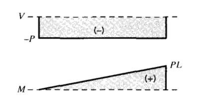
As stated earlier, the stresses and defflections will be shown to be functions of \(V\) and \(M\), so it is important to be able to compute how these quantities vary along the beam's length. Plots of \(V(x)\) and \(M(x)\) are known as shear and bending moment diagrams, and it is necessary to obtain them before the stresses can be determined. For the end-loaded cantilever, the diagrams shown in Figure 3 are obvious from Eqns. 4.1.1 and 4.1.2.
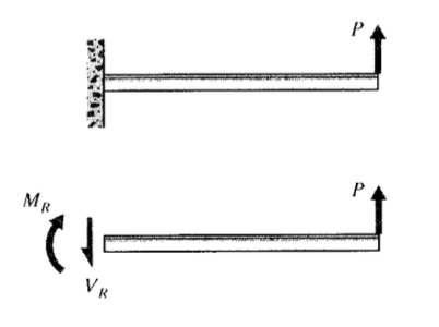
It was easiest to analyze the cantilevered beam by beginning at the free end, but the choice of origin is arbitrary. It is not always possible to guess the easiest way to proceed, so consider what would have happened if the origin were placed at the wall as in Figure 4. Now when a free body diagram is constructed, forces must be placed at the origin to replace the reactions that were imposed by the wall to keep the beam in equilibrium with the applied load. These reactions can be determined from free-body diagrams of the beam as a whole (if the beam is statically determinate), and must be found before the problem can proceed. For the beam of Figure 4:
\(\sum F_y = 0 = -V_R + P \Rightarrow V_R = P\)
The shear and bending moment at \(x\) are then
\(V(x) = V_R = P = \text{constant}\)
This choice of origin produces some extra algebra, but the \(V(x)\) and \(M(x)\) diagrams shown in Figure 5 are the same as before (except for changes of sign): \(V\) is constant and equal to \(P\), and \(M\) varies linearly from zero at the free end to \(PL\) at the wall.
Distributed loads
Transverse loads may be applied to beams in a distributed rather than at-a-point manner as depicted in Figure 6, which might be visualized as sand piled on the beam. It is convenient to describe these distributed loads in terms of force per unit length, so that \(q(x)\) would be the load applied to a small section of length \(dx\) by a distributed load \(q(x)\). The shear force \(V(x)\) set up in reaction to such a load is
\[V(x) = - \int_{x_0}^{x} q(\xi) d \xi\]
Figure 5: Alternative shear and bending moment diagrams for the cantilevered beam.
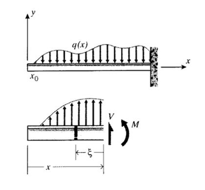
where \(x_0\) is the value of \(x\) at which \q(x)\) begins, and \(\xi\) is a dummy length variable that looks backward from \(x\). Hence \(V(x)\) is the area under the \(q(x)\) diagram up to position \(x\). The moment balance is obtained considering the increment of load \(q(\xi) d \xi\) applied to a small width \(d \xi\) of beam, a distance \(\xi\) from point \(x\). The incremental moment of this load around point \(x\) is \(q(\xi) \xi d \xi\), so the moment \(M(x)\) is
\[M = \int_{x_0}^{x} q(\xi) \xi d \xi\]
This can be related to the centroid of the area under the \(q(x)\) curve up to \(x\), whose distance from \(x\) is
\(\bar{\xi} = \dfrac{\int q(\xi) \xi d \xi}{\int q (\xi) d\xi}\)
Hence Equation 4.1.4 can be written
\[M = Q \bar{\xi}\]
where \(Q = \int q (\xi) d\xi\) is the area. Therefore, the distributed load \(q(x)\) is statically equivalent to a concentrated load of magnitude \(Q\) placed at the centroid of the area under the \(q(x)\) diagram.
Example \(\PageIndex{1}\)
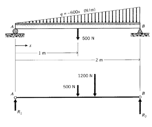
Consider a simply-supported beam carrying a triangular and a concentrated load as shown in Figure 7. For the purpose of determining the support reaction forces \(R_1\) and \(R_2\), the distributed triangular load can be replaced by its static equivalent. The magnitude of this equivalent force is
The equivalent force acts through the centroid of the triangular area, which is 2/3 of the distance from its narrow end (see Exercis \(\PageIndex{1}\)). The reaction \(R_2\) can now be found by taking moments around the left end:
The other reaction can then be found from vertical equilibrium:
Successive integration method
Figure 8: Relations between distributed loads and internal shear forces and bending moments.
We have already noted in Equation 4.1.3 that the shear curve is the negative integral of the loading curve. Another way of developing this is to consider a free body balance on a small increment of length \(dx\) over which the shear and moment changes from \(V\) and \(M\) to \(V + dV\) and \(M + dM\) (see Figure 8). The distributed load \(q(x)\) can be taken as constant over the small interval, so the force balance is:
\[\dfrac{dV}{dx} = -q\]
or
\[V(x) = - \int q(x) \ dx\]
which is equivalent to Equation 4.1.3. A moment balance around the center of the increment gives
As the increment \(dx\) is reduced to the limit, the term containing the higher-order differential \(dV\ dx\) vanishes in comparison with the others, leaving
\[\dfrac{dM}{dx} = -V\]
or
\[M(x) = -\int V(x)\ dx\]
Hence the value of the shear curve at any axial location along the beam is equal to the negative of the slope of the moment curve at that point, and the value of the moment curve at any point is equal to the negative of the area under the shear curve up to that point.
The shear and moment curves can be obtained by successive integration of the \(q(x)\) distribution, as illustrated in the following example.
Example \(\PageIndex{2}\)
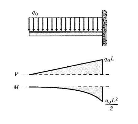
Consider a cantilevered beam subjected to a negative distributed load \(q(x) = -q_0\) = constant as shown in Figure 9; then
\(V(x) = -\int q(x)\ dx = q_0 x + c_1\)
where \(c_1\) is a constant of integration. A free body diagram of a small sliver of length near \(x = 0\) shows that \(V(0) = 0\), so the \(c_1\) must be zero as well. The moment function is obtained by integrating again:
\(M(x) = -\int V(x) \ dx = -\dfrac{1}{2} q_0 x^2 + c_2\)
where \(c_2\) is another constant of integration that is also zero, since \(M(0) = 0\).
Admittedly, this problem was easy because we picked one with null boundary conditions, and with only one loading segment. When concentrated or distributed loads are found at different
positions along the beam, it is necessary to integrate over each section between loads separately. Each integration will produce an unknown constant, and these must be determined by invoking the continuity of slopes and defflections from section to section. This is a laborious process, but one that can be made much easier using singularity functions that will be introduced shortly.
It is often possible to sketch \(V\) and \(M\) diagrams without actually drawing free body diagrams or writing equilibrium equations. This is made easier because the curves are integrals or derivatives of one another, so graphical sketching can take advantage of relations among slopes and areas.
These rules can be used to work gradually from the \(q(x)\) curve to \(V(x)\) and then to \(M(x)\). Wherever a concentrated load appears on the beam, the \(V(x)\) curve must jump by that value, but in the opposite direction; similarly, the \(M(x)\) curve must jump discontinuously wherever a couple is applied to the beam.
Example \(\PageIndex{3}\)
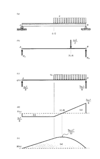
To illustrate this process, consider a simply-supported beam of length \(L\) as shown in Figure 10, loaded over half its length by a negative distributed load \(q = -q_0\). The solution for \(V(x)\) and \(M(x)\) takes the following steps:
1. The reactions at the supports are found from static equilibrium. Replacing the distributed load by a concentrated load \(Q = -q_0 (L/2)\) at the midpoint of the \(q\) distribution (Figure 10(b))and taking moments around \(A\):
\(R_B L = (\dfrac{q_0L}{2}) (\dfrac{3L}{4}) \Rightarrow R_B = \dfrac{3q_0L}{8}\)
The reaction at the right end is then found from a vertical force balance:
Note that only two equilibrium equations were available, since a horizontal force balance would provide no relevant information. Hence the beam will be statically indeterminate if more than two supports are present.
The \(q(x)\) diagram is then just the beam with the end reactions shown in Figure 10(c).
2. Beginning the shear diagram at the left, \(V\) immediately jumps down to a value of \(-q_0 L/8\) in opposition to the discontinuously applied reaction force at \(A\); it remains at this value until \(x = L/2\) as shown in Figure 10(d).
3. At \(x = L/2\), the \(V(x)\) curve starts to rise with a constant slope of \(+ q_0\) as the area under the \(q(x)\) distribution begins to accumulate. When \(x = L\), the shear curve will have risen by an amount \(q_0 L/2\), the total area under the \(q(x)\) curve; its value is then \((-q_0 l/8) + (q_0 L/2) = (3q_0 L/8)\). The shear curve then drops to zero in opposition to the reaction force \(R_B = (3q_0 L/8)\). (The \(V\) and \(M\) diagrams should always close, and this provides a check on the work.)
4. The moment diagram starts from zero as shown in Figure 10(e), since there is no discontinuously applied moment at the left end. It moves upward at a constant slope of \(+q_0L/8\), the value of the shear diagram in the first half of the beam. When \(x = L/2\), it will have risen to a value of \(q_0 L^2/16\).
5. After \(x = L/2\), the slope of the moment diagram starts to fall as the value of the shear diagram rises. The moment diagram is now parabolic, always being one order higher than the shear diagram. The shear diagram crosses the \(V = 0\) axis at \(x = 5L/8\), and at this point the slope of the moment diagram will have dropped to zero. The maximum value of \(M\) is \(9q_0 L^2/32\), the total area under the \(V\) curve up to this point.
6. After \(x = 5L/8\), the moment diagram falls parabolically, reaching zero at \(x = L\).
Singularity functions
This special family of functions provides an automatic way of handling the irregularities of loading that usually occur in beam problems. They are much like conventional polynomial factors, but with the property of being zero until "activated" at desired points along the beam. The formal definition is
\[f_n (x) = \langle x - a \rangle^n = \begin{cases} 0, & x < a \\ (x - a)^n, & x > a \end{cases}\]
where \(n = -2, -1, 0, 1, 2, \cdots\). The function \(\langle x - a \rangle^0\) is a unit step function, \(\langle x - a \rangle_{-1}\) is a concentrated load, and \(\langle x - a \rangle_{-2}\) is a concentrated couple. The first five of these functions are sketched in Figure 11.
Figure 11: Singularity functions.
The singularity functions are integrated much like conventional polynomials:
\[\int_{-\infty}^{x} \langle x - a \rangle^n \ dx = \dfrac{\langle x - a \rangle^{n+1}}{n + 1} \ n \ge 0\]
However, there are special integration rules for the \(n = -1\) and \(n = -2\) members, and this special handling is emphasized by using subscripts for the \(n\) index:
\[\int_{\infty}^{x} \langle x - a \rangle_{-2}\ dx = \langle x - a \rangle_{-1}\]
\[\int_{\infty}^{x} \langle x - a \rangle_{-1}\ dx = \langle x - a \rangle^0\]
Example \(\PageIndex{4}\)
Applying singularity functions to the beam of Example 4.3, the loading function would be written
The reaction force at the right end could also be included, but it becomes activated only as the problem is over. Integrating once:
The constant of integration is included automatically here, since the influence of the reaction at \(A\) has been included explicitly. Integrating again:
Examination of this result will show that it is the same as that developed previously.
Maple\(^{\text{TM}}\) symbolic manipulation software provides an efficient means of plotting these functions. The following shows how the moment equation of this example might be plotted, using the Heaviside function to provide the singularity.
# Define function sfn in terms of a and n
>sfn:=proc(a,n) (x-a)^n*Heaviside(x-a) end;
      sfn := proc(a, n) (x - a)^n*Heaviside(x - a) end proc
# Input moment equation using singularity functions
>M(x):=(q*L/8)*sfn(0,1)-(q/2)*sfn(L/2,2);
  M(x) := 1/8 q L x Heaviside(x) 2
        -1/2q(x-1/2L) Heaviside(x-1/2L)
# Provide numerical values for q and L: >q:=1: L:=10:
# Plot function >plot(M(x),x=0..10);
Figure 12: Maple singularity plot
Exercise \(\PageIndex{1}\)
(a)-(c) Locate the magnitude and position of the force equivalent to the loading distributions shown here.
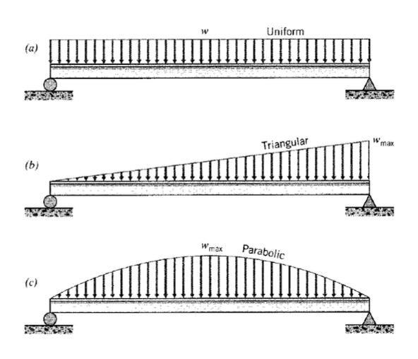
Exercise \(\PageIndex{2}\)
(a)- (c) Determine the reaction forces at the supports of the cases in Exercise \(\PageIndex{1}\).
Exercise \(\PageIndex{3}\)
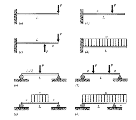
(a)-(h) Sketch the shear and bending moment diagrams for the load cases shown here.
Exercise \(\PageIndex{4}\)
(a)-(h) Write singularity-function expressions for the shear and bending moment distributions for the cases in Exercise \(\PageIndex{3}\).
Exercise \(\PageIndex{5}\)
(a)-(h) Use Maple (or other) software to plot the shear and bending moment distributions for the cases in Exercise \(\PageIndex{3}\), using the values (as needed) \(L = 25 \ in, a = 5\ in, w = 10\ lb/in, P = 150 \ lb\).
Exercise \(\PageIndex{6}\)
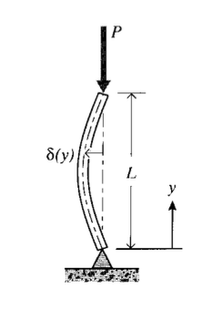
The transverse deflecti \(n\) of a beam under an axial load \(P\) is taken to be \(\delta (y) = \delta_0 \sin (y \pi /L)\), as shown here. Determine the bending moment \(M(y)\) along the beam.
Exercise \(\PageIndex{7}\)
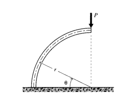
Determine the bending moment \(M(\theta)\) along the circular curved beam shown.