6.1: Yield and Plastic Flow

Introduction

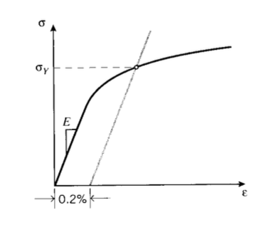
In our overview of the tensile stress-strain curve in Module 4, we described yield as a permanent molecular rearrangement that begins at a sufficiently high stress, denoted \(\sigma_Y\) in Figure 1. The yielding process is very material-dependent, being related directly to molecular mobility. It is often possible to control the yielding process by optimizing the materials processing in a way that influences mobility. General purpose polystyrene, for instance, is a weak and brittle plastic often credited with giving plastics a reputation for shoddiness that plagued the industry for years. This occurs because polystyrene at room temperature has so little molecular mobility that it experiences brittle fracture at stresses less than those needed to induce yield with its associated ductile flow. But when that same material is blended with rubber particles of suitable size and composition, it becomes so tough that it is used for batting helmets and ultra-durable children’s toys. This magic is done by control of the yielding process. Yield control to balance strength against toughness is one of the most important aspects of materials engineering for structural applications, and all engineers should be aware of the possibilities.

Figure 1: Yield stress \(\sigma_Y\) as determined by the 0.2% offset method.

Another important reason for understanding yield is more prosaic: if the material is not allowed to yield, it is not likely to fail. This is not true of brittle materials such as ceramics that fracture before they yield, but in most of the tougher structural materials no damage occurs before yield. It is common design practice to size the structure so as to keep the stresses in the elastic range, short of yield by a suitable safety factor. We therefore need to be able to predict when yielding will occur in general multidimensional stress states, given an experimental value of \(\sigma_Y\).

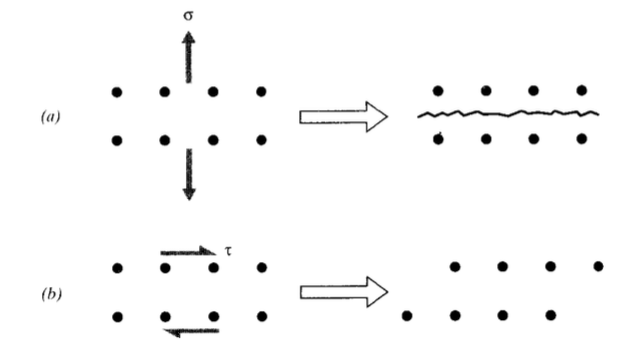
Fracture is driven by normal stresses, acting to separate one atomic plane from another. Yield, conversely, is driven by shearing stresses, sliding one plane along another. These two distinct mechanisms are illustrated n Figure 2. Of course, bonds must be broken during the sliding associated with yield, but unlike in fracture are allowed to reform in new positions. This process can generate substantial change in the material, even leading eventually to fracture (as in bending a metal rod back and forth repeatedly to break it). The "plastic" deformation that underlies yielding is essentially a viscous flow process, and follows kinetic laws quite similar to liquids. Like flow in liquids, plastic flow usually takes place without change in volume, corresponding to Poisson’s ratio \(ν = 1/2\).

Figure 2: Cracking is caused by normal stresses (a), sliding is caused by shear stresses (b).

Multiaxial stress states

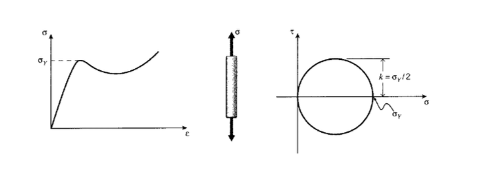
The yield stress \(\sigma_Y\) is usually determined in a tensile test, where a single uniaxial stress acts. However, the engineer must be able to predict when yield will occur in more complicated real-life situations involving multiaxial stresses. This is done by use of a yield criterion, an observation derived from experimental evidence as to just what it is about the stress state that causes yield. One of the simplest of these criteria, known as the maximum shear stress or Tresca criterion, states that yield occurs when the maximum shear stress reaches a critical value \(\tau_{\max} = k\). The numerical value of \(k\) for a given material could be determined directly in a pure-shear test, such as torsion of a circular shaft, but it can also be found indirectly from the tension test as well. As shown in Figure 3, Mohr’s circle shows that the maximum shear stress acts on a plane \(45^{\circ}\) away from the tensile axis, and is half the tensile stress in magnitude; then \(k = \sigma_Y/2\).

In cases of plane stress, Mohr’s circle gives the maximum shear stress in that plane as half the difference of the principal stresses:

\[\tau_{\max} = \dfrac{\sigma_{p1} - \sigma_{p2}}{2}\]

Figure 3: Mohr’s circle construction for yield in uniaxial tension.

Example \(\PageIndex{1}\)

Using \(\sigma_{p1} = \sigma_{\theta} = pr/b\) and \(\sigma_{p2} = \sigma_{z} = pr/2b\) in 6.1.1, the shear stress in a cylindrial pressure vessel with closed ends is (See Module 6)

 

where the \(\theta_z\) subscript indicates a shear stress in a plane tangential to the vessel wall. Based on this, we might expect the pressure vessel to yield when

\(\tau_{\max , \theta_z} = k = \dfrac{sigma_Y}{2}\)

which would occur at a pressure of

\(p_Y = \dfrac{4b\tau{\max , \theta_z}}{r} \overset{?}{=} \dfrac{2b\sigma_Y}{r}\)

However, this analysis is in error, as can be seen by drawing Mohr’s circles not only for the \(\theta_z\) plane but for the \(\theta_r\) and \(rz\) planes as well as shown in Figure 4.

Figure 4: Principal stresses and Mohr’s circle for closed-end pressure vessel

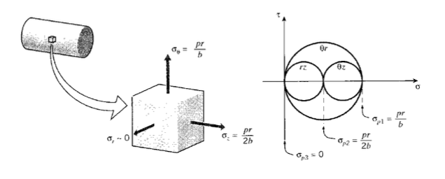
The shear stresses in the \(\theta_r\) plane are seen to be twice those in the \(\theta_z\) plane, since in the \(\theta_r\) plane the second principal stress is zero:

 

Yield will therefore occur in the \(\theta_r\) plane at a pressure of \(b\sigma_Y/r\), half the value needed to cause yield in the \(\theta_z\) plane. Failing to consider the shear stresses acting in this third direction would lead to a seriously underdesigned vessel.

Situations similar to this example occur in plane stress whenever the principal stresses in the \(xy\) plane are of the same sign (both tensile or both compressive). The maximum shear stress, which controls yield, is half the difference between the principal stresses; if they are both of the same sign, an even larger shear stress will occur on the perpendicular plane containing the larger of the principal stresses in the xy plane.

This concept can be used to draw a “yield locus” as shown in Figure 5, an envelope in \(\sigma_1 - \sigma_2\) coordinates outside of which yield is predicted. This locus obviously crosses the coordinate axes at values corresponding to the tensile yield stress \(\sigma_Y\). In the I and III quadrants the principal stresses are of the same sign, so according to the maximum shear stress criterion yield is determined by the difference between the larger principal stress and zero. In the II and IV quadrants the locus is given by \(\tau_{\max} = |\sigma_1 - \sigma_2|/2 = \sigma_Y /2\), so \(\sigma_1 - \sigma_2\) = const; this gives straight diagonal lines running from \(\sigma_Y\) on one axis to \(\sigma_Y\) on the other.

Figure 5. Yield locus for the maximum-shear stress criterion.

Example \(\PageIndex{2}\)

Figure 6: (a) Circular shaft subjected to simultaneous twisting and tension. (b) Mohr’s circle construction.

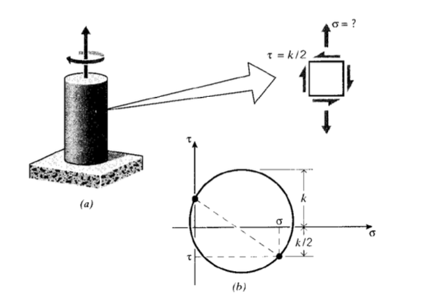
A circular shaft is subjected to a torque of half that needed to cause yielding as shown in Figure 6; we now ask what tensile stress could be applied simultaneously without causing yield.

A Mohr's circle is drawn with shear stress \(\tau = k/2\) and unknown tensile stress \(\sigma\). Using the Tresca maximum-shear yield criterion, yield will occur when \(\sigma\) is such that

\(\tau_{\max} = k = \sqrt{(\dfrac{\sigma}{2})^2 + (\dfrac{k}{2})^2}\)

\(\sigma = \sqrt{3} k\)

The Tresca criterion is convenient to use in practice, but a somewhat better fit to experi- mental data can often be obtained from the “von Mises” criterion, in which the driving force for yield is the strain energy associated with the deviatoric components of stress. The von Mises stress (also called the equivalent or effective stress) is defined as

 

In terms of the principal stresses this is

 

where the stress differences in parentheses are proportional to the maximum shear stresses on the three principal planes(Some authors use a factor other than 1/2 within the radical. This is immaterial, since it will be absorbed by the calculation of the critical value of \(\sigma_M\)) (Since the quantities are squared, the order of stresses inside the parentheses is unimportant.) The Mises stress can also be written in compact form in terms of the second invariant of the deviatoric stress tensor \(\Sigma_{ij}\):

\[\sigma_M = \sqrt{3\Sigma_{ij} \Sigma_{ij}/2}\]

It can be shown that this is proportional to the total distortional strain energy in the material, and also to the shear stress τoct on the "octahedral" plane oriented equally to the 1-2-3 axes. The von Mises stress is the driving force for damage in many ductile engineering materials, and is routinely computed by most commercial finite element stress analysis codes.

The value of von Mises stress \(\sigma_{M,Y}\) needed to cause yield can be determined from the tensile yield stress \(\sigma_Y\), since in tension at the yield point we have \(\sigma_1 = \sigma_Y\), \(\sigma_2 = \sigma_3 = 0\). Then

 

Hence the value of von Mises stress needed to cause yield is the same as the simple tensile yield stress.

The shear yield stress \(k\) can similarly be found by inserting the principal stresses corresponding to a state of pure shear in the Mises equation. Using \(k = \sigma_1 = -\sigma_3\) and \(\sigma_2 = 0\), we have

 

\(k = \dfrac{\sigma_Y}{\sqrt{3}}\)

Note that this result is different than the Tresca case, in which we had \(k = \sigma_Y/2\).

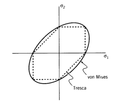
The von Mises criterion can be plotted as a yield locus as well. Just as the Tresca criterion, it must pass through \(\sigma_Y\) on each axis. However, it plots as an ellipse rather than the prismatic shape of the Tresca criterion (see Figure 7).

Figure 7: Yield locus for the von Mises criterion.

Effect of hydrostatic pressure

Since in the discussion up to now yield has been governed only by shear stress, it has not mattered whether a uniaxial stress is compressive or tensile; yield occurs when \(\sigma = \pm \sigma_Y\). This corresponds to the hydrostatic component of the stress \(-p = (\sigma_x + \sigma_y + \sigma_z)/3\) having no influence on yield, which is observed experimentally to be valid for slip in metallic systems. Polymers, however, are much more resistant to yielding in compressive stress states than in tension. The atomistic motions underlying slip in polymers can be viewed as requiring "free volume" as the molecular segments move, and this free volume is diminished by compressive stresses. It is thus difficult to form solid polymers by deformation processing such as stamping and forging in the same way steel can be shaped; this is one reason the vast majority of automobile body panels continue to be made of steel rather than plastic.

Figure 8: Effect of pressure on the von Mises yield envelope.

This dependency on hydrostatic stress can be modeled by modifying the yield criterion to state that yield occurs when

\[\tau_{\max} \text{ or } \sigma_M \ge r_0 + A_p\]

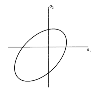
where \(\tau_0\) and \(A\) are constants. As \(p\) increases (the hydrostatic component of stress becomes more positive) the shear stress needed for yield becomes greater as well, since there is less free volume and more hindrance to molecular motion. The effect of this modification is to slide the von Mises ellipse to extend less into the I quadrant and more into the III quadrant as shown in Figure 8. This shows graphically that greater stresses are needed for yield in compression, and lesser stresses in tension.

Figure 9: A craze in polystyrene (from R. Kambour, “Crazing,” Encyclopedia of Polymer Science and Engineering, Wiley-Interscience, 1991).

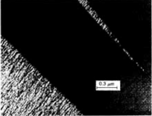
Several amorphous glassy polymers — notably polystyrene, polymethylmethacrylate, and polycarbonate — are subject to a yield mechanism termed "crazing" in which long elongated voids are created within the material by a tensile cavitation process. Figure 9 shows a craze in polystyrene, grown in plasticizing fluid near \(T_g\). The voids, or crazes, are approximately 1000A thick and microns or more in length, and appear visually to be much like conventional

cracks. They differ from cracks, however, in that the broad faces of the crazes are spanned by a great many elongated fibrils that have been drawn from the polymer as the craze opens. The fibril formation requires shear flow, but the process is also very dependent on free volume. A successful multiaxial stress criterion for crazing that incorporates both these features has been proposed(S. Sternstein and L. Ongchin, Polymer Preprints, 10, 1117, 1969.) of the form

 

The left hand side of this relation is proportional to the shear stress, and the denominator in the second term on the right hand side is related to the hydrostatic component of the stress. As the hydrostatic tension increases, the shear needed to cause crazing decreases. The parameters \(A\) and \(B\) are adjustable, and both depend on temperature. This relation plots as a batwing on the yield locus diagram as seen in Figure 10, approaching a \(45^{\circ}\) diagonal drawn through the II and IV quadrants. Crazing occurs to the right of the curve; note that crazing never occurs in compressive stress fields.

Figure 10: The Sternstein envelopes for crazing and pressure-inhibited shear yielding.

Crazing is a yield mechanism, but it also precipitates brittle fracture as the craze height increases and the fibrils are brought to rupture. The point where the craze locus crosses the shear yielding locus is therefore a type of mechanically induced ductile-brittle transition, as the failure mode switches from shear yielding to craze embrittlement. Environmental agents such as acetone that expand the free volume in these polymers greatly exacerbate the tendency for craze brittleness. Conversely, modifications such as rubber particle inclusions that stabilize the crazes and prevent them from becoming true cracks can provide remarkable toughness. Rubber particles not only stabilize crazes, they also cause a great increase in the number of crazes, so the energy absorption of craze formation can add to the toughness as well. This is the basis of the “high impact polystyrene,” or HIPS, mentioned at the outset of this chapter.

Effect of rate and temperature

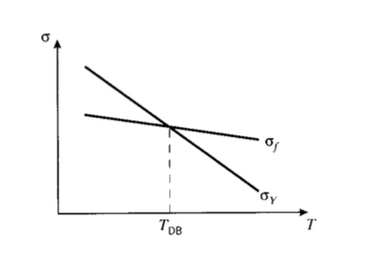
The yield process can be viewed as competing with fracture, and whichever process has the lowest stress requirements will dominate. As the material is made less and less mobile, for instance by lowering the temperature or increasing the number and tightness of chemical bonds, yielding becomes more and more difficult. The fracture process is usually much less dependent on mobility. Both yield and fracture stresses usually increase with decreasing temperature, but yield is more temperature-dependent (see Figure 11). This implies that below a critical temperature (called the ductile-brittle transition temperature TDB) the material will fracture before it yields. Several notable failures in ships and pipelines have occurred during winter temperatures when the steels used in their manufacture were stressed below their TDB and were thus unable to resist catastrophic crack growth. In polymers, the ductile-brittle transition temperature is often coincident with the glass transition temperature. Clearly, we need an engineering model capable of showing how yield depends on temperature, and one popular approach is outlined below.

Yield processes are thermally activated, stress driven motions, much like the flow of viscous liquids. Even without going into much detail as to the specifics of the motions, it is possible to write down quite effective expressions for the dependency of these motions on strain rate and temperature. In the Eyring view of thermally activated processes, an energy barrier \(E_Y^*\) must be overcome for the motion to proceed. (We shall use the asterisk superscript to indicate activation

Figure 11: Schematic illustration of the temperature dependence of yield and fracture stress.

parameters, and the \(Y\) subscript here indicates the yield process.) A stress acts to lower the barrier when it acts in the direction of flow, and to raise it when it opposes the flow.

Consider now a constant strain rate test (\(\dot{\epsilon}\) = const), in which the stress rises until yield occurs at \(\sigma = \sigma_Y\). At the yield point we have \(d\sigma/d\epsilon = 0\), so a fluidlike state is achieved in which an increment of strain can occur without a corresponding incremental increase in stress. Analogously with rate theories for viscous flow, an Eyring rate equation can be written for the yielding process as

\[\dot{\epsilon} = \dot{\epsilon_0} \exp \dfrac{-(E_Y^* - \sigma_Y V^*)}{kT}\]

Here \(k\) is Boltzman’s constant and \(V^*\) is a factor governing the effectiveness of the stress in reducing the activation barrier. It must have units of volume for the product \(\sigma_Y V^*\) to have units of energy, and is called the "activation volume" of the process. Taking logs and rearranging,

\(\dfrac{\sigma_Y}{T} = \dfrac{E_Y^*}{V*T} + \dfrac{k}{V^*} \ln \left(\dfrac{\dot{\epsilon}}{\dot{\epsilon_0}}\right)\)

Hence plots of \(\sigma_Y/T\) versus \(\ln \dot{\epsilon}\) should be linear with a slope \(k/V^*\) as seen in Figure 12, from which the activation volume may be computed. The horizontal spacing between two lines at differing temperatures \(T_1\) and \(T_2\) gives the activation energy:

 

Apparent activation volumes in polymers are on the order of 5000 \(\dot{A}\), much larger than a single repeat unit. This is taken to indicate that yield in polymers involves the cooperative motion of several hundred repeat units.

Example \(\PageIndex{3}\)

The yield stress for polycarbonate is reported at 60 MPa at room-temperature (\(23^{\circ}C\) = \(296^{\circ}K\)), and we wish to know its value at \(0^{\circ}C\) (273\(^{\circ}K\)), keeping the strain rate the same.

This can be accomplished by writing Equation 4 out twice, once for each temperature, and then dividing one by the other. The parameters \(\dot{\epsilon}\) and \(\dot{\epsilon_0}\) cancel, leaving

 

From the data in Figure 12, the yield activation parameters are \(E_Y^* = 309\ kJ/mol\), \(V^* = 3.9 \times 10^{-3}\ m^3/mol\). Using these along with \(R = 8.314\ J/mol\) and \(\sigma_Y^{296} = 60 \times 10^6\ N/m^2\), we have

Figure 12: Eyring plot showing dependence of yield strength on temperature and strain rate in polycarbonate (from N.G. McCrum, C.P Buckley and C.B. Bucknall, Principles of Polymer Engineering, Oxford University Press, 1988).

\(\sigma_Y^{273} = 61.5\ MPa\)

Continuum plasticity

Plasticity theory, which seeks to determine stresses and displacements in structures all or part of which have been stressed beyond the yield point, is an important aspect of solid mechanics. The situation is both materially and geometrically nonlinear, so it is not a trivial undertaking. However, in such areas as metal forming, plasticity theory has provided valuable insight. We will outline only a few aspects of this field in the following paragraphs, to introduce some of the fundamental concepts that the reader can extend in future study.

Plastic deformation

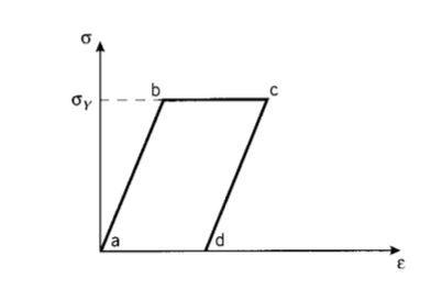
A useful idealization in modeling plastic behavior takes the material to be linearly elastic up to the yield point as shown in Figure 13, and then “perfectly plastic” at strains beyond yield. Strains up to yield (the line between points \(a\) and \(b\)) are recoverable, and the material unloads along the same elastic line it followed during loading; this is conventional elastic response. But if the material is strained beyond yield (point \(b\)), the "plastic" straining beyond b takes place at constant stress and is unrecoverable. If the material is strained to point \(c\) and then unloaded, it follows the path cd (a line parallel to the original elastic line \(ab\)) rather than returning along \(cba\). When the stress has been brought to zero (point \(d\)), the plastic strain ad remains as a residual strain.

Figure 13: The elastic-perfectly plastic idealization of plastic deformation.

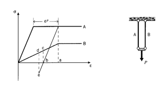
Plastic deformation can generate "residual" stresses in structures, internal stresses that remain even after the external loads are removed. To illustrate this, consider two rods having different stress-strain curves, connected in parallel (so their strains are always equal) as shown in Figure 14. When the rods are strained up to the yield point of rod B (point a on the strain axis), rod \(A\) will have experienced an amount of permanent plastic deformation \(\epsilon^p\). When the applied load is removed, rod \(B\) unloads along its original stress-strain curve, but rod \(A\) follows a path parallel to its original elastic line. When rod \(A\) reaches zero stress (point \(b\)), rod \(B\) will still be in tension (point \(c\)). In order for the load transmitted by the rods together to come to zero, rod \(B\) will pull rod \(A\) into compression until \(-\sigma_B = -\sigma_A\) as indicated by points \(d\) and \(e\). Residual stresses are left in the rods, and the assembly as a whole is left with a residual tensile strain.

Figure 14: Plastic deformation of two-bar assembly.

Compressive residual stress can be valuable if the structure must bear tensile loads. Similarly to how rapid quenching can be used to make safety glass by putting the surfaces in compression, plastic deformation can be used to create favorable compressive stresses. One famous such technique is called “autofrettage;” this is a method used to strengthen cannon barrels against bursting by pressurizing them from the inside so as to bring the inner portion of the barrel into the plastic range. When the pressure is removed, the inner portions are left with a compressive residual stress just as with bar \(A\) in the above example.

Wire drawing

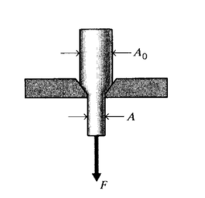
To quantify the plastic flow process in more detail, consider next the "drawing" of wire(G.W. Rowe, Elements of Metalworking Theory, Edward Arnold, London, 1979.), in which wire is pulled through a reducing die so as to reduce its cross-sectional area from \(A_0\) to \(A\) as shown in Figure 15. Since volume is conserved during plastic deformation, this corresponds to an axial elongation of \(L/L_0 = A_0/A\). Considering the stress state to be simple uniaxial tension, we have

Figure 15: Wire drawing.

\(\sigma_1 = \sigma_Y, \sigma_2 = \sigma_3 = 0\)

where 1 denotes the direction along the wire and 2 and 3 are the transverse directions. The work done in stretching the wire by an increment of length dL, per unit volume of material, is

\(dU = \dfrac{dW}{AL} = \dfrac{\sigma_Y A dL}{AL}\)

Integrating this from \(L_0\) to \(L\) to obtain the total work:

\(U = \int_{L_0}^{L} dU = \dfrac{FdL}{AL} = \sigma_Y \ln \dfrac{L}{L_0}\)

The quantity \(ln(L/L_0)\) is the logarithmic strain \(\epsilon_T\) introduced in Module 4 (Stress-Strain Curves).

Example \(\PageIndex{1}\)

The logarithmic strain can be written in terms of either length increase or area reduction, due to the constancy of volume during plastic deformation: \(\epsilon_T = \ln (L/L_0) = \ln (A_0/A)\). In terms of diameter reduction, the relation \(A = \pi d^2/4\) leads to

\(e_T = \ln (\dfrac{\pi d_0^2/4}{\pi d^2/4}) = 2\ln (\dfrac{d_0}{d})\)

Taking the pearlite cell size to shrink commensurately with the diameter, we expect the wire strength \(\sigma_f\) to vary according to the Hall-Petch relation with \(1/\sqrt{d}\). The relation between wire strength and logarithmic drawing strain is then

\(\sigma_f \propto \dfrac{\exp (\epsilon_T/4)}{\sqrt{d_0}}\)

The work done by the constant pulling force \(F\) in drawing an initial length \(L_0\) of wire to a new length \(L\) is \(W = FL\). This must equal the work per unit volume done in the die, multiplied by the total volume of wire:

\(FL = (AL) \sigma_Y \ln \dfrac{L}{L_0}\)

Written in terms of area reduction, this is

\(F = A \sigma_Y \ln \dfrac{A_0}{A}\)

This simple result is useful in estimating the requirements of wire drawing, even though it neglects the actual complicated flow field within the die and the influence of friction at the die walls. Both friction at the surface and constraints to flow within the field raise the force needed in drawing, but the present analysis serves to establish a lower-limit approximation. It is often written in terms of the drawing stress \(\sigma_1 = F/A\) and the area reduction ratio \(r = (A_0 - A)/A_0 = 1 - (A/A_0)\):

 

Note that the draw stress for a small area reduction is less than the tensile yield stress. In fact, the maximum area reduction that can be achieved in a single pass can be estimated by solving for the value of \(r\) which brings the draw stress up to the value of the yield stress, which it obviously cannot exceed. This calculation gives

 

Hence the maximum area reduction is approximately 63%, assuming perfect lubrication at the die. This lower-bound treatment gives an optimistic result, but is not far from the approximately 50% reduction often used as a practical limit. If the material hardens during drawing, the maximum reduction can be slightly greater.

Slip-line fields

In cases of plane strain, there is a graphical technique called slip-line theory(W. Johnson and P.B. Mellor, Plasticity for Mechanical Engineers, Van Nostrand Co., New York, 1962.) which permits a more detailed examination of plastic flow fields and the loads needed to create them. Friction and internal flow constraints can be included, so upper-bound approximations are obtained that provide more conservative estimates of the forces needed in deformation. Considerable experience is needed to become proficient in this method, but the following will outline some of the basic ideas.

Consider plane strain in the 1-3 plane, with no strain in the 2-direction. There is a Poisson stress in the 2-direction, given by

 

Since \(v = 1/2\) in plastic flow,

\(\sigma_2 = \dfrac{1}{2} (\sigma_1 + \sigma_3)\)

The hydrostatic component of stress is then

\(p = \dfrac{1}{3} (\sigma_1 + \sigma_2 + \sigma_3) = \dfrac{1}{2} (\sigma_1 + \sigma_3) = \sigma_2\)

Hence the Poisson stress \(\sigma_2\) in the zero-strain direction is the average of the other two stresses \(\sigma_1\) and \(\sigma_2\), and also equal to the hydrostatic component of stress. The stress state can be specified in terms of the maximum shear stress, which is just \(k\) during plastic flow, and the superimposed hydrostatic pressure \(p\):

\(\sigma_1 = -p + k\), \(\sigma_2 = -p\), \(\sigma_3 = -p -k\)

Since the shear stress is equal to \(k\) everywhere, the problem is one of determining the directions of \(k\) (the direction of maximum shear, along which slip occurs), and the magnitude of \(p\).

The graphical technique involves sketching lines that lie along the directions of \(k\). Since maximum shear stresses act on two orthogonal planes, there will be two sets of these lines, always perpendicular to one another and referred to as \(\alpha\)-lines and \(\beta\)-lines. The direction of these lines is specified by an inclination angle \(\phi\). Any convenient inclination can be used for the \(\phi = 0\) datum, and the identification of \(\alpha\)- vs. \(\beta\)-lines is such as to make the shear stress positive according to the usual convention. As the pressure \(p\) varies from point to point, there is a corresponding variation of the angle \(\phi\), given by the Hencky equations as

\(p + 2k\phi = C_1 =\) constant, along an \(\alpha\)-line

 

Hence the pressure can be determined from the curvature of the sliplines, once the constant is known.

The slip-line field must obey certain constraints at boundaries:

1. Free surfaces: Since there can be no stress normal to a free surface, we can put \(\sigma_3 = 0\) there and then

\(p = k, \sigma_1 = -p -k = -2k\)

Hence the pressure is known to be just the shear yield strength at a free surface. Further- more, since the directions normal and tangential to the surface are principal directions, the directions of maximum shear must be inclined at \(45^{\circ}\) to the surface.

2. Frictionless surface: The shear stress must be zero tangential to a frictionless surface, which again means that the tangential and normal directions must be principal directions. Hence the slip lines must meet the surface at \(45^{\circ}\). However, there will in general be a stress acting normal to the surface, so \(\sigma_3 \ne 0\) and thus \(p\) will not be equal to \(k\).

3. Perfectly rough surface: If the friction is so high as to prevent any tangential motion at the surface, the shearing must be maximum in a direction that is also tangential to the surface. One set of slip lines must then be tangential to the surface, and the other set normal to it.

Figure 16: Slip-line construction for a flat indentation.

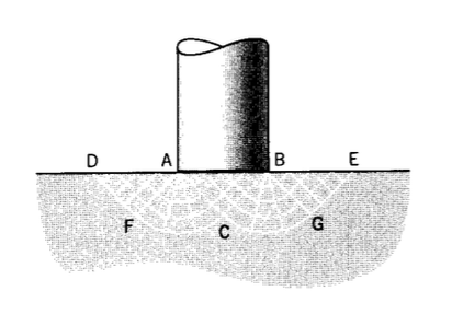
Consider a flat indentor of width b being pressed into a semi-infinite block, with negligible friction (see Figure 16). Since the sliplines must meet the indentor surface at \(45^{\circ}\), we can draw a triangular flow field \(ABC\). Since all lines in this region are straight, there can be no variation in the pressure \(p\), and the field is one of "constant state." This cannot be the full extent of the field, however, since it would be constrained both vertically and laterally by rigid metal. The field must extend to the free surfaces adjacent to the punch, so that downward motion under the punch can be compensated by upward flow adjacent to it. Two more triangular regions \(ADF\) and \(BEG\) are added that satisfy the boundary conditions at free surfaces, and these are connected to the central triangular regions by "fans" \(AFC\) and \(BCG\). Fans are very useful in slip-line constructions; they are typically centered on singularities such as points \(A\) and \(B\) where there is no defined normal to the surface.

The pressure on the punch needed to establish this field can be determined from the sliplines, and this is one of their principal uses. Since BE is a free surface, \(\sigma_3 = 0\) there and \(p = k\). The pressure remains constant along line \(EG\) since \(\phi\) is unchanging, but as \(\phi\) decreases along the curve \(GC\) (the line curves clockwise), the pressure must increase according to the Hencky equation. At point \(C\) it has rotated through \(-\pi/2\) so the pressure there is

\(p_C + 2k\phi = p_C + 2k (-\dfrac{\pi}{2}) =\) constant = \(p_G = k\)

\(p_C = k(1 +\pi)\)

The pressure remains unchanged along lines \(CA\) and \(CB\), so the pressure along the punch face is also \(k(1 + \pi)\). The total stress acting upward on the punch face is therefore

\(\sigma_1 = p +k =2k(1 + \dfrac{\pi}{2})\)

The ratio of punch pressure to the tensile yield strength \(2k\) is

\(\dfrac{\sigma_1}{2k} = 1 + \dfrac{\pi}{2} = 2.571\)

The factor 2.571 represents the increase over the tensile yield strength caused by the geometrical constraints on the flow field under the punch.

The Brinell Hardness Test is similar to the punch yielding scenario above, but uses a hard steel sphere instead of a flat indentor. The Brinell hardness \(H\) is calculated as the load applied to the punch divided by the projected area of the indentation. Analysis of the Brinell test differs somewhat in geometry, but produces a result not much different than that of the flat punch:

 

This relation is very useful in estimating the yield strength of metals by simple nondestructive indentation hardness tests.

Exercise \(\PageIndex{1}\)

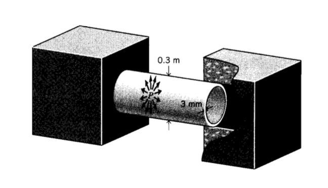
An open-ended pressure vessel is constructed of aluminum, with diameter 0.3 m and wall thickness 3 mm. (Open-ended in this context means that both ends of the vessel are connected to other structural parts able to sustain pressure, as in a hose connected between two reservoirs.) Determine the internal pressure at which the vessel will yield according to the (a) Tresca and (b) von Mises criteria.

Exercise \(\PageIndex{2}\)

Repeat the previous problem, but with the pressure vessel now being closed-ended.

Exercise \(\PageIndex{3}\)

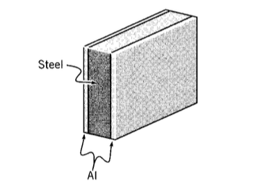
A steel plate is clad with a thin layer of aluminum on both sides at room temperature, and the temperature then raised. At what temperature increase \(\Delta T\) will the aluminum yield?

Exercise \(\PageIndex{4}\)

If the temperature in the previous problem is raised \(40\{circ} C\) beyond the value at which yielding occurs, and is thereafter lowered back to room temperature, what is the residual stress left in the aluminum?

Exercise \(\PageIndex{5}\)

Copper alloy is subjected to the stress state \(\sigma_x = 100\), \(\sigma_y = -200\), \(\tau_{xy} = 100\) (all in MPa). Determine whether yield will occur according to the (a) Tresca and (b) von Mises criterion.

Exercise \(\PageIndex{6}\)

Repeat the previous problem, but with the stress state \(\sigma_x = 190\), \(\sigma_y = 90\), \(\tau_{xy} = 120\) (all in MPa).

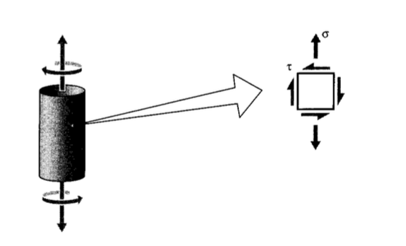
Exercise \(\PageIndex{7}\)

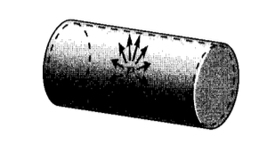
A thin-walled tube is placed in simultaneous tension and torsion, causing a stress state as shown here. Construct a plot of \(\tau /\sigma_Y\) vs. \(\sigma /\sigma_Y\) at which yield will occur according to the (a) Tresca and (b) von Mises criterion. (\(\sigma\) is the tensile yield stress.)

Exercise \(\PageIndex{8}\)

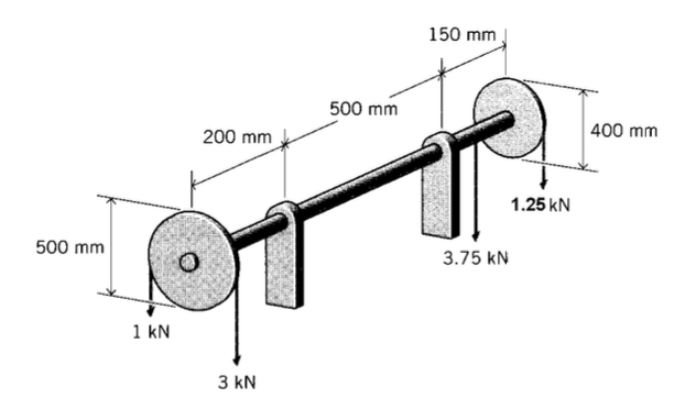
A solid circular steel shaft is loaded by belt pulleys at both ends as shown. Determine the diameter of the shaft required to avoid yield according to the von Mises criterion, with a factor of safety of 2.

Exercise \(\PageIndex{9}\)

For polycarbonate, the kinetic parameters in 6.1.4 are found to be are \(\dot{\epsilon_0} = 448 s^{-1}\), \(E_Y^* = 309\ kJ/mol\), and \(V* = 3.9 \times 10^{-3}\ m^3/mol\). Find the yield stress \(\sigma_Y\) at a strain rate of \(\dot{\epsilon} = 10^2 s^{-1}\) and temperature \(40^{\circ}C\).

Exercise \(\PageIndex{10}\)

Yield stresses (in MPa) have been measured at various strain rates and temperatures as follows:

	\(\dot{epsilon} = 10^{-3} s^{-1}\)	\(\dot{epsilon} = 10^{-1} s^{-1}\)
\(T = 0^{\circ} C\)	54.1	62.7
\(T = 40^{\circ} C\)	42.3	52.1

Determine the activation volume for the yield process. What physical significance might this parameter have?

Exercise \(\PageIndex{11}\)

The yield stress of a polymer is measured to be 20 MPa at a temperature of 300K and a strain rate of \(10^{-3}s^{-1}\). When the strain rate is doubled from this value, the yield stress is observed to increase by 10%. What is the apparent activation volume for yield in this case?

Exercise \(\PageIndex{12}\)

Show the von Mises stress can be written in index notation as \(\sigma_M = \sqrt{3 \Sigma_{ij} \Sigma_{ij}/2}\)

Exercise \(\PageIndex{13}\)

A sample of linear polyethylene was tested in uniaxial loading at \(T = 23^{\circ} C\) and \(\dot{\epsilon} = 10^{-3}s^{-1}\). The yield stress \(\sigma_Y\) was found to be 30.0 MPa in tension and 31.5 MPa in compression. Determine the pressure-dependency constant \(A\) in Equation 3.

Exercise \(\PageIndex{14}\)

A circular shaft of radius R is subjected to a torque \(T\).

(a) What value of \(T\) will be just large enough to induce yielding at the outer surface?

(b) As the value of \(T\) is increased beyond the level found in (a), determine the radius re within which the material is still in the elastic range.

(c) What value of \(T\) will make the shaft fully plastic; i.e. \(r_e = 0\)?

Exercise \(\PageIndex{15}\)

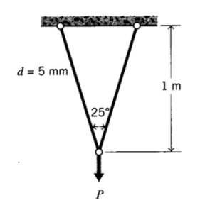
A two-element truss frame is constructed of steel with the geometry shown. What load \(P\) can the frame support without yielding in either element?

Exercise \(\PageIndex{16}\)

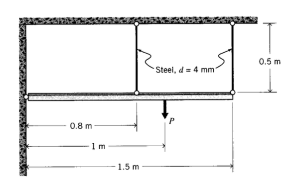
A three-element truss frame is constructed of steel with the geometry shown. What load \(P\) can the frame support before all three elements have yielded?

Exercise \(\PageIndex{17}\)

If the frame of the previous problem is loaded until all three members have yielded and the load then reduced to zero, find the residual stress in the central element.

Exercise \(\PageIndex{18}\)

A rigid beam is hinged at one end as shown and supported by two vertical rods as shown.

(a) What load \(P\) can the structure support before both vertical rods have yielded?
(b) What is the residual stress in the vertical rods after the load has been reduced to zero?

Exercise \(\PageIndex{19}\)

Estimate the drawing force required to reduce the diameter of a \(0.125''\) aluminum rod by 50% in a wire-drawing operation.