6.3: Statistics of Fracture
- Page ID
- 44552

Introduction
One particularly troublesome aspect of fracture, especially in high-strength and brittle materials, is its variability. The designer must be able to cope with this, and limit stresses to those which reduce the probability of failure to an acceptably low level. Selection of an acceptable level of risk is a difficult design decision itself, obviously being as close to zero as possible in cases where human safety is involved but higher in doorknobs and other inexpensive items where failure is not too much more than a nuisance. The following sections will not replace a thorough study of statistics, but will introduce at least some of the basic aspects of statistical theory needed in design against fracture. The text by Collins(Collins, J.A., Failure of Materials in Mechanical Design, Wiley, 1993.) includes an extended treatment of statistical analysis of fracture and fatigue data, and is recommended for further reading.
Basic Statistical Measures
The value of tensile strength \(\sigma_f\) cited in materials property handbooks is usually the arithmetic mean, simply the sum of a number of individual strength measurements divided by the number of specimens tested:
\[\overline{\sigma_f} = \dfrac{1}{N} \sum_{i = 1}^{N} \sigma_{f,i}\]
where the overline denotes the mean and \(\sigma_f, i\) is the measured strength of the \(i^{th}\) (out of \(N\)) individual specimen. Of course, not all specimens have strengths exactly equal to the mean; some are weaker, some are stronger. There are several measures of how widely scattered is the distribution of strengths, one important one being the sample standard deviation, a sort of root mean square average of the individual deviations from the mean:
\[s = \sqrt{\dfrac{1}{N-1} \sum_{i = 1}^{N} (\overline{\sigma_f} - \sigma_{x,i})^2}\]
The significance of \(s\) to the designer is usually in relation to how large it is compared to the mean, so the coefficient of variation, or C.V., is commonly used:
\(\text{C.V.} = \dfrac{s}{\overline{\sigma_f}}\)
This is often expressed as a percentage. Coefficients of variation for tensile strength are commonly in the range of 1–10%, with values much over that indicating substantial inconsistency in the specimen preparation or experimental error.
Example \(\PageIndex{1}\)
In order to illustrate the statistical methods to be outlined in this Module, we will use a sequence of thirty measurements of the room-temperature tensile strength of a graphite/epoxy composite(P. Shyprykevich, ASTM STP 1003, pp. 111–135, 1989.). These data (in kpsi) are: 72.5, 73.8, 68.1, 77.9, 65.5, 73.23, 71.17, 79.92, 65.67, 74.28, 67.95, 82.84, 79.83, 80.52, 70.65, 72.85, 77.81, 72.29, 75.78, 67.03, 72.85, 77.81, 75.33, 71.75, 72.28, 79.08, 71.04, 67.84, 69.2, 71.53. Another thirty measurements from the same source, but taken at 93\(^{\circ} C\) and -59\(^{\circ} C\), are given in Probs. 2 and 3, and can be subjected to the same treatments as homework.
There are several computer packages available for doing statistical calculations, and most of the procedures to be outlined here can be done with spreadsheets. The Microsoft Excel functions for mean and standard deviation are average() and stdev(), where the arguments are the range of cells containing the data. These give for the above data
\(\overline{\sigma_f} = 73.28, \ \ \ s = 4.63 \text{ (kpsi)}\)
The coefficient of variation is \(\text{C.V.} = (4.63/73.28) \times 100% = 6.32%\).
The Normal Distribution
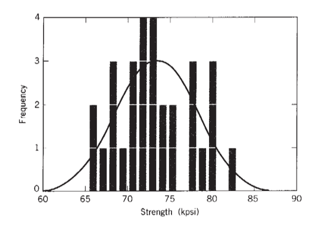
A more complete picture of strength variability is obtained if the number of individual specimen strengths falling in a discrete strength interval \(\Delta \sigma_f\) is plotted versus σf in a histogram as shown in Figure 1; the maximum in the histogram will be near the mean strength and its width will be related to the standard deviation.
As the number of specimens increases, the histogram can be drawn with increasingly finer \(\Delta \sigma_f\) increments, eventually forming a smooth probability distribution function, or "pdf". The mathematical form of this function is up to the material (and also the test method in some cases) to decide, but many phenomena in nature can be described satisfactorily by the normal, or Gaussian, function:
\[f(X) = \dfrac{1}{\sqrt{2\pi}} \exp \dfrac{-X^2}{2}, \ \ \ X = \dfrac{\sigma_f - \overline{\sigma_f}}{s}\]
Here \(X\) is the standard normal variable, and is simply how many standard deviations an individual specimen strength is away from the mean. The factor \(1/\sqrt{2 \pi}\) normalizes the function so that its integral is unity, which is necessary if the specimen is to have a 100% chance of failing at some stress. In this expression we have assumed that the measure of standard deviation determined from Equation 6.3.2 based on a discrete number of specimens is acceptably close to the "true" value that would be obtained if every piece of material in the universe could somehow be tested.
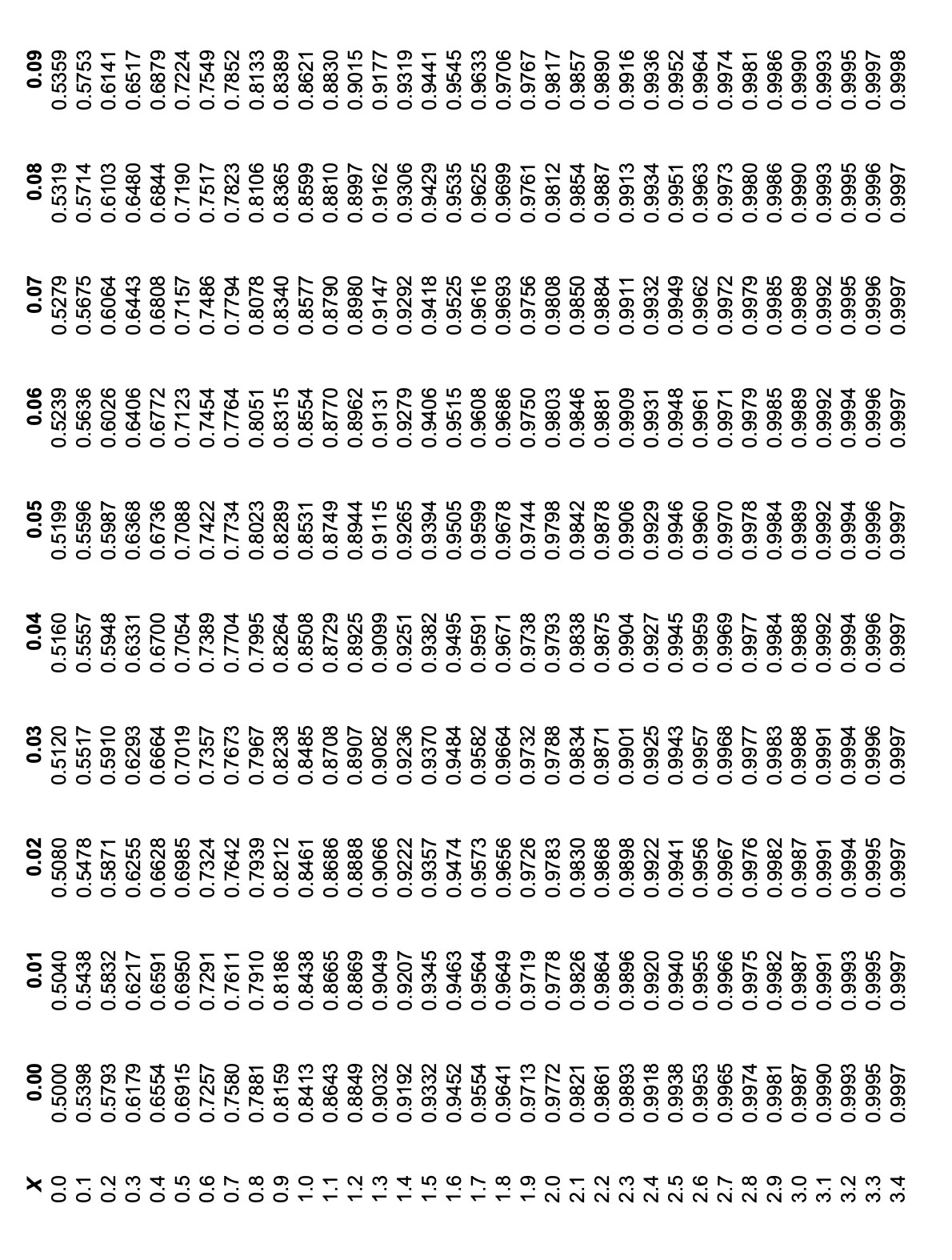
The normal distribution function \(f(X)\) plots as the “bell curve” familiar to all grade- conscious students. Its integral, known as the cumulative distribution function or \(P_f(X)\), is also used commonly; its ordinate is the probability of fracture, also the fraction of specimens having a strength lower than the associated abscissal value. Since the normal pdf has been normalized, the cumulative function rises with an S-shaped or sigmoidal shape to approach unity at large values of \(X\). The two functions \(f(X)\) and \(F(X)\) are plotted in Figure 2, and tabulated in Tables 1 and 2 of the Appendix attached to this module. (Often the probability of survival \(P_s = 1−P_f\) is used as well; this curve begins at near unity and falls in a sigmoidal shape toward zero as the applied stress increases.)
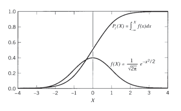
Figure 2: Differential \(f(X)\) and cumulative \(P_f(X)\) normal probability functions.
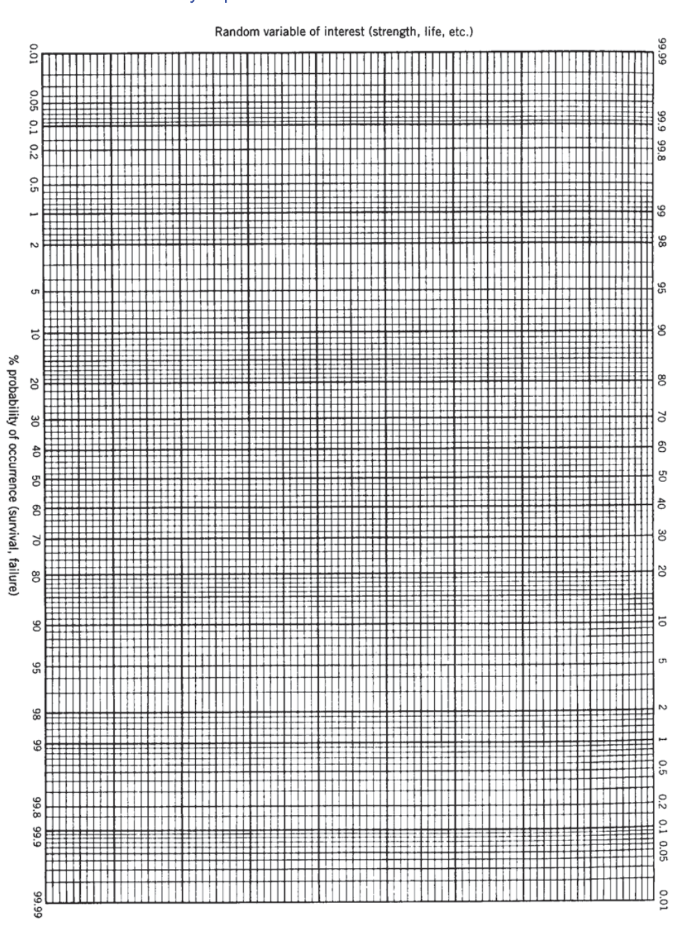
One convenient means of determining whether or not a particular set of measurements is normally distributed involves using special graph paper (a copy is included in the Appendix) whose ordinate has been distorted to make the sigmoidal cumulative distribution Pf plot as a straight line. (Sometimes it is easier to work with straight lines on curvy paper than curvy lines on straight paper.) Experimental data are ranked from lowest to highest, and each assigned a rank based on the fraction of strengths having higher values. If the ranks are assigned as i/(N + 1), where i is the position of a datum in the ordered list and N is the number of specimens, the ranks are always greater than zero and less than one; this facilitates plotting.
The degree to which these rank-strength data plot as straight lines on normal probability paper is then a visual measure of how well the data are described by a normal distribution. The best-fit straight line through the points passes the 50% cumulative fraction line at the sample mean, and its slope gives the standard distribution. Plotting several of these lines, for instance for different processing conditions of a given material, is a convenient way to characterize the strength differences arising from the two conditions (See Prob. 2).
Example \(\PageIndex{2}\)
For our thirty-specimen test population, the ordered and ranked data are:
| \(i\) | \(\sigma_{f,i}\) | \(P_f = \dfrac{i}{N+1}\) |
|---|---|---|
| 1 | 65.50 | 0.0323 |
| 2 | 65.67 | 0.0645 |
| 3 | 67.03 | 0.0968 |
| 4 | 67.84 | 0.1290 |
| 5 | 67.95 | 0.1613 |
| 6 | 68.10 | 0.1935 |
| 7 | 69.20 | 0.2258 |
| 8 | 70.65 | 0.2581 |
| 9 | 71.04 | 0.2903 |
| 10 | 71.17 | 0.3226 |
| 11 | 71.53 | 0.3548 |
| 12 | 71.75 | 0.3871 |
| 13 | 72.28 | 0.4194 |
| 14 | 72.29 | 0.4516 |
| 15 | 72.5 | 0.4839 |
| 16 | 72.85 | 0.5161 |
| 17 | 72.85 | 0.5484 |
| 18 | 72.23 | 0.5806 |
| 19 | 73.80 | 0.6129 |
| 20 | 74.28 | 0.6452 |
| 21 | 75.33 | 0.6774 |
| 22 | 75.78 | 0.7097 |
| 23 | 77.81 | 0.7419 |
| 24 | 77.81 | 0.7742 |
| 25 | 77.90 | 0.8065 |
| 26 | 79.08 | 0.8387 |
| 27 | 79.83 | 0.8710 |
| 28 | 79.92 | 0.9032 |
| 29 | 80.52 | 0.9355 |
| 30 | 82.84 | 0.9677 |
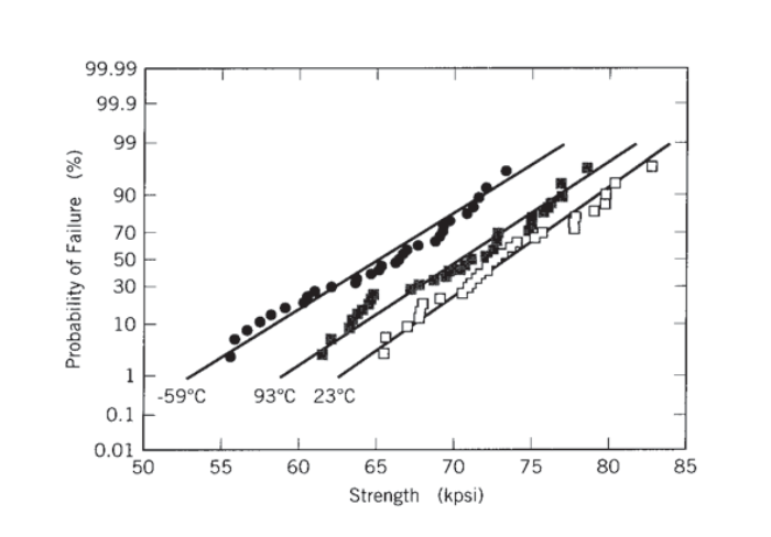
When these are plotted using probability scaling on the ordinate, the graph in Figure 3 is obtained.
The normal distribution function has been characterized thoroughly, and it is possible to infer a great deal of information from it for strength distributions that are close to normal. For instance, the cumulative normal distribution function (cdf) tabulated in Table 2 of the Appendix shows that that 68.3% of all members of a normal distribution lie within \(\pm 1s\) of the mean, 95% lie within \(\pm\)1.96s, and 99.865% lie within \(\pm 3s\). It is common practice in much aircraft design to take \(\overline{\sigma_f} - 3s\) as the safe fracture fracture strength; then almost 99.9% of all specimens will have a strength at least this high. This doesn’t really mean one out of every thousand airplane wings are unsafe; within the accuracy of the theory, 0.1% is a negligible number, and the 3\(s\) tolerance includes essentially the entire population("Six-sigma" has become a popular goal in manufacturing, which means that only one part out of approximately a billion will fail to meet specification.). Having to reduce the average strength by \(3s\) in design can be a real penalty for advanced materials such as composites that have high strengths but also high variability due to their processing methods being relatively undeveloped. This is a major factor limiting the market share of these advanced materials.
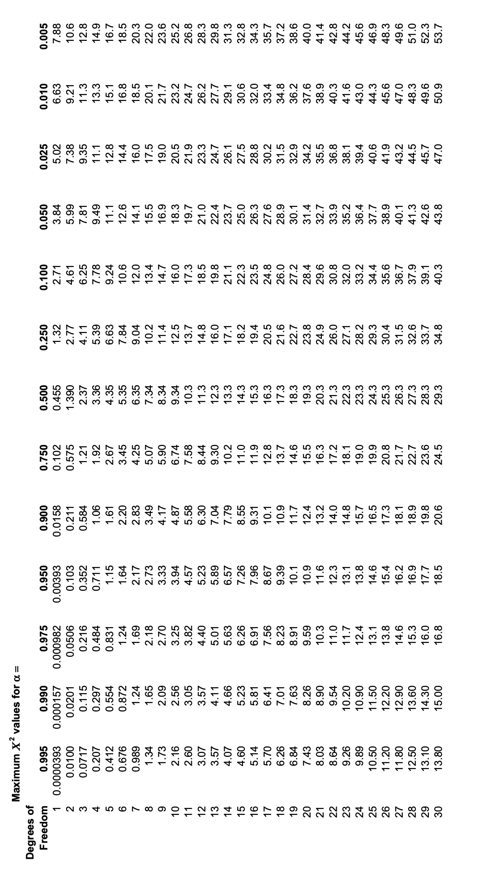
Beyond the visual check of the linearity of the probability plot, several "goodness-of-fit" tests are available to assess the degree to which the population can reasonably be defined by the normal (or some other) distribution function. The "Chi-square" test is often used for this purpose. Here a test statistic measuring how far the observed data deviate from those expected from a normal distribution, or any other proposed distribution, is
where \(n_i\) is the number of specimens actually failing in a strength increment \(\Delta \sigma_{f,i}, N\) is the total number of specimens, and \(p_i\) is the probability expected from the assumed distribution of a specimen having having a strength in that increment.
Example \(\PageIndex{3}\)
To apply the Chi-square test to our 30-test population, we begin by counting the number of strengths falling in selected strength increments, much as if we were constructing a histogram. We choose five increments to obtain reasonable counts in each increment. The number expected to fall in each increment is determined from the normal pdf table, and the square of the difference calculated.
| Lower Limit | Upper Limit | Observed Frequency | Expected Frequency | Chisquare |
|---|---|---|---|---|
| 0 | 69.33 | 7 | 5.9 | 0.198 |
| 69.33 | 72.00 | 5 | 5.8 | 0.116 |
| 72.00 | 74.67 | 8 | 6.8 | 0.214 |
| 74.67 | 77.33 | 2 | 5.7 | 2.441 |
| 77.33 | \(\infty\) | 8 | 5.7 | 0.909 |
| \(\chi^2 = 3.878\) |
The number of degrees of freedom for this Chi-square test is 4; this is the number of increments less one, since we have the constraint that \(n_1 + n_2 + n_3 + n_5 = 30\).
Interpolating in the Chi-Square Distribution Table (Table 3 in the Appendix), we find that a fraction 0.44 of normally distributed populations can be expected to have \(\chi^2\) statistics of up to 3.88. Hence, it seems reasonable that our population can be viewed as normally distributed.
Usually, we ask the question the other way around: is the computed \(\chi^2\) so large that only a small fraction - say 5% - of normally distributed populations would have \(\chi^2\) values that high or larger? If so, we would reject the hypothesis that our population is normally distributed.
From the \(\chi^2\) Table, we read that \(\alpha = 0.05\) for \(\chi^2 = 9.488\), where \(\alpha\) is the fraction of the \(\chi^2\) population with values of \(\chi^2\) greater than 9.488. Equivalently, values of \(\chi^2\) above 9.488 would imply that there is less than a 5% chance that a population described by a normal distribution would have the computed \(\chi^2\) value. Our value of 3.878 is substantially less than this, and we are justified in claiming our data to be normally distributed.
Several governmental and voluntary standards-making organizations have worked to develop standardized procedures for generating statistically allowable property values for design of critical structures(Military Handbook 17B, Army Materials Technology Laboratory, Part I, Vol. 1, 1987.). One such procedure defines the "B-allowable" strength as that level for which we have 95% confidence that 90% of all specimens will have at least that strength. (The use of two percentages here may be confusing. We mean that if we were to measure the strengths of 100 groups each containing 10 specimens, at least 95 of these groups would have at least 9 specimens whose strengths exceed the B-allowable.) In the event the normal distribution function is found to provide a suitable description of the population, the B-basis value can be computed from the mean and standard deviation using the formula
where \(k_b\) is \(n^{-1/2}\) times the 95th quantile of the “noncentral t-distribution;” this factor is tabulated, but can be approximated by the formula
Example \(\PageIndex{4}\)
In the case of the previous 30-test example, \(k_B\) is computed to be 1.78, so this is less conservative than the \(3s\) guide. The B-basis value is then
Having a distribution function available lets us say something about the confidence we can have in how reliably we have measured the mean strength, based on a necessarily limited number of individual strength tests. A famous and extremely useful result in mathematical statistics states that, if the mean of a distribution is measured \(N\) times, the distribution of the means will have its own standard deviation \(s_m\) that is related to the mean of the underlying distribution \(s\) and the number of determinations, \(N\) as
\[s_m = \dfrac{s}{\sqrt{N}}\]
This result can be used to establish confidence limits. Since 95% of all measurements of a normally distributed population lie within 1.96 standard deviations from the mean, the ratio \(\pm 1.96s/\sqrt{N}\)
is the range over which we can expect 95 out of 100 measurements of the mean to
fall. So even in the presence of substantial variability we can obtain measures of mean strength to any desired level of confidence; we simply make more measurements to increase the value of \(N\) in the above relation. The "error bars" often seen in graphs of experimental data are not always labeled, and the reader must be somewhat cautious: they are usually standard deviations, but they may indicate maximum and minimum values, and occasionally they are 95% confidence limits. The significance of these three is obviously quite different.
Example \(\PageIndex{5}\)
Equation 6.3.4 tells us that were we to repeat the 30-test sequence of the previous example over and over (obviously with new specimens each time), 95% of the measured sample means would lie within the interval
\(73.278 - \dfrac{(1.96)(4.632)}{\sqrt{30}}, 73.278 + \dfrac{(1.96)(4.632)}{\sqrt{30}} = 71.62, 74.94\)
The \(t\) distribution
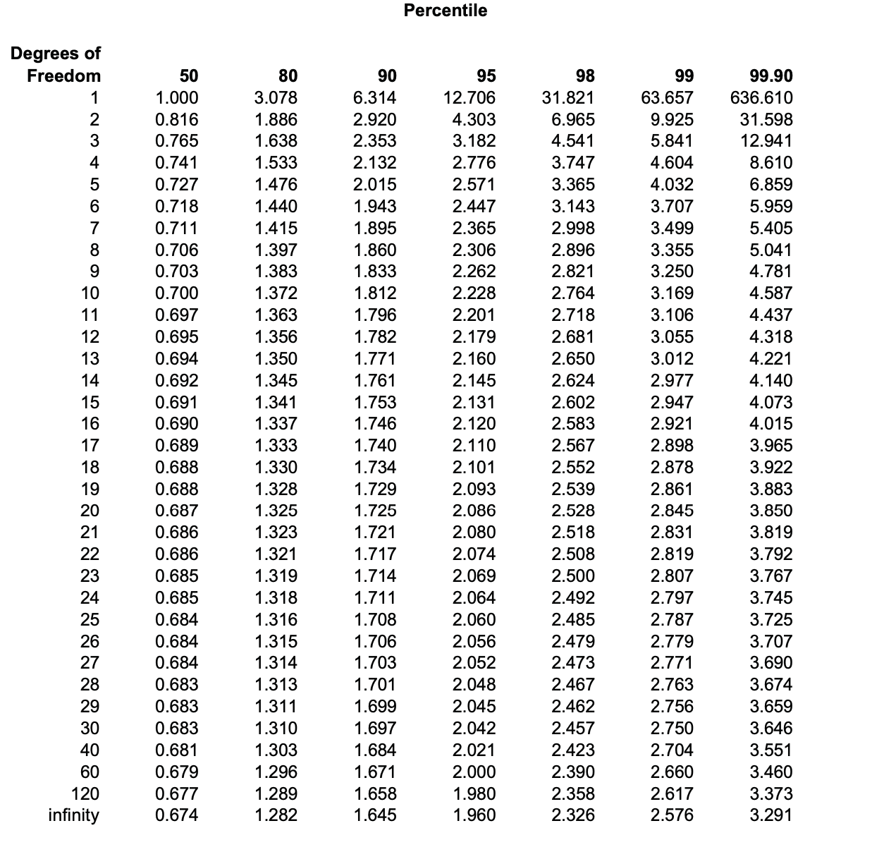
The "\(t\)" distribution, tabulated in Table 4 of the Appendix, is similar to the normal distribution, plotting as a bell-shaped curve centered on the mean. It has several useful applications to strength data. When there are few specimens in the sample, the t-distribution should be used in preference to the normal distribution in computing confidence limits. As seen in the table, the t-value for the 95th percentile and the 29 degrees of freedom of our 30-test sample in Example 6.3.3 is 2.045. (The number of degrees of freedom is one less than the total specimen count, since the sum of the number of specimens having each recorded strength is constrained to be the total number of specimens.) The 2.045 factor replaces 1.96 in this example, without much change in the computed confidence limits. As the number of specimens increases, the t-value approaches 1.96. For fewer specimens the factor deviates substantially from 1.96; it is 2.571 for \(n = 5\) and 3.182 for \(n = 3\).
The \(t\) distribution is also useful in deciding whether two test samplings indicate significant differences in the populations they are drawn from, or whether any difference in, say, the means of the two samplings can be ascribed to expected statistical variation in what are two essentially identical populations. For instance, Figure 3 shows the cumulative failure probability for graphite- epoxy specimens tested at three different temperatures, and it appears that the mean strength is reduced somewhat by high temperatures and even more by low temperatures. But are these differences real, or merely statistical scatter?
This question can be answered by computing a value for \(t\) using the means and standard deviations of any two of the samples, according to the formula
\[t = \dfrac{|\bar{\sigma} f_1 - \bar{\sigma} f_2|}{\sqrt{\dfrac{s_1^2}{n_1 - 1} + \dfrac{s_2^2}{n_2 - 1}}}\]
This statistic is known to have a \(t\) distribution if the deviations \(s_1\) and \(s_2\) are not too different. The mean and standard deviation of the \(-59^{\circ} C\) data shown in Figure 3 are 65.03 and 5.24 respec- tively. Using Equation 5 to compare the room-temperature (\(23^{\circ} C\)) and \(-59^{\circ} C\) data, the \(t\)-statistic is
\(t = \dfrac{(73.28 - 65.03)}{\sqrt{\dfrac{(4.63)^2}{29} + \dfrac{(5.24)^2}{29}}} = 6.354\)
From Table 4 in the Appendix, we now look up the value of \(t\) for 29 degrees of freedom corresponding to 95% (or some other value, as desired) of the population. We do this by scanning the column for \(F(t) = 0.975\) rather than 0.95, since the \(t\) distribution is symmetric and another 0.025 fraction of the population lies beyond \(t = -0.975\). The \(t\) value for 95% \((F(t) = 0.975)\) and 29 degrees of freedom is 2.045.
This result means that were we to select repeatedly any two arbitrary 30-specimen samples from a single population, 95% of these selections would have t-statistics as computed with Equation 6.3.5 less than 2.045; only 5% would produce larger values of \(t\). Since the 6.354 t-statistic for the \(-59^{\circ}C\) and 23\(^{\circ} C\) samplings is much greater than 2.045, we can conclude that it is very unlikely that the two sets of data are from the same population. Conversely, we conclude that the two datasets are in fact statistically independent, and that temperature has a statistically significant effect on the strength.
The Weibull distribution
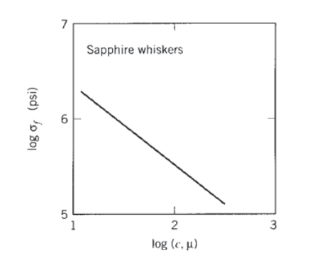
Large specimens tend to have lower average strengths than small ones, simply because large ones are more likely to contain a flaw large enough to induce fracture at a given applied stress. This effect can be measured directly, for instance by plotting the strengths of fibers versus the fiber circumference as in Figure 4. For similar reasons, brittle materials tend to have higher strengths when tested in flexure than in tension, since in flexure the stresses are concentrated in a smaller region near the outer surfaces.
The hypothesis of the size effect led to substantial development effort in the statistical analysis community of the 1930's and 40's, with perhaps the most noted contribution being that of W. Weibull(See B. Epstein, J. Appl. Phys., Vol. 19, p. 140, 1948 for a useful review of the statistical treatment of the size effect in fracture, and for a summary of extreme-value statistics as applied to fracture problems.) in 1939. Weibull postulated that the probability of survival at a stress \(\sigma\), i.e. the probability that the specimen volume does not contain a flaw large enough to fail under the stress \(\sigma\), could be written in the form
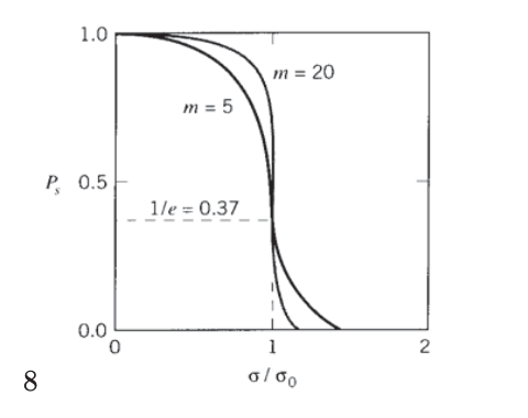
\[P_s(\sigma) = \exp [-(\dfrac{\sigma}{\sigma_0})^m]\]
Weibull selected the form of this expression for its mathematical convenience rather than some fundamental understanding, but it has been found over many trials to describe fracture statistics well. The parameters \(\sigma_0\) and \(m\) are adjustable constants; Figure 5 shows the form of the Weibull function for two values of the parameter \(m\). Materials with greater variability have smaller values of \(m\); steels have \(m \approx 100\), while ceramics have \(m \approx 10\). This parameter can be related to the coefficient of variation; to a reasonable approximation, \(m \approx 1.2/C.V.\)
A variation on the normal probability paper graphical method outlined earlier can be developed by taking logarithms of Equation 6.3.6:
\(\begin{array} {rcl} {\ln P_s} & = & {-(\dfrac{\sigma}{\sigma_0})^m} \\ {\ln (\ln P_s)} & = & {-m \ln (\dfrac{\sigma}{\sigma_0})} \end{array}\)
Hence the double logarithm of the probability of exceeding a particular strength \(\sigma\) versus the logarithm of the strength should plot as a straight line with slope \(m\).
Example \(\PageIndex{6}\)
Again using the 30-test sample of the previous examples, an estimate of the \(\sigma_0\) parameter can be obtained by plotting the survival probability (1 minus the rank) and noting the value of σf at which Ps drops to \(1/e = 0.37\); this gives \(\sigma_0 \approx 74\). (A more accurate regression method gives 75.46.) A tabulation of the double logarithm of \(P_s\) against the logarithm of \(\sigma_f/\sigma_0\) is then
| \(i\) | \(\sigma_{f,i}\) | \(\ln \ln (1/P_s)\) | \(\ln (\sigma_{f,i}/\sigma_0)\) |
|---|---|---|---|
| 1 | 65.50 | -3.4176 | -0.1416 |
| 2 | 65.67 | -2.7077 | -0.1390 |
| 3 | 67.03 | -2.2849 | -0.1185 |
| 4 | 67.84 | -1.9794 | -0.1065 |
| 5 | 67.95 | -1.7379 | -0.1048 |
| 6 | 68.10 | -1.5366 | -0.1026 |
| 7 | 69.20 | -1.3628 | -0.0866 |
| 8 | 70.65 | -1.2090 | -0.0659 |
| 9 | 71.04 | -1.0702 | -0.0604 |
| 10 | 71.17 | -0.9430 | -0.0585 |
| 11 | 71.53 | -0.8250 | -0.0535 |
| 12 | 71.75 | -0.7143 | -0.0504 |
| 13 | 72.28 | -0.6095 | -0.0431 |
| 14 | 72.29 | -0.5095 | -0.0429 |
| 15 | 72.50 | -0.4134 | -0.0400 |
| 16 | 72.85 | -0.3203 | -0.0352 |
| 17 | 72.85 | -0.2295 | -0.0352 |
| 18 | 73.23 | -0.1404 | -0.0300 |
| 19 | 73.80 | -0.0523 | -0.0222 |
| 20 | 74.28 | 0.0355 | -0.0158 |
| 21 | 75.33 | 0.1235 | -0.0017 |
| 22 | 75.78 | 0.2125 | 0.0042 |
| 23 | 77.81 | 0.3035 | 0.0307 |
| 24 | 77.81 | 0.3975 | 0.0307 |
| 25 | 77.90 | 0.4961 | 0.0318 |
| 26 | 79.08 | 0.6013 | 0.0469 |
| 27 | 79.83 | 0.7167 | 0.0563 |
| 28 | 79.92 | 0.8482 | 0.0574 |
| 29 | 80.52 | 1.0083 | 0.0649 |
| 30 | 82.84 | 1.2337 | 0.0933 |
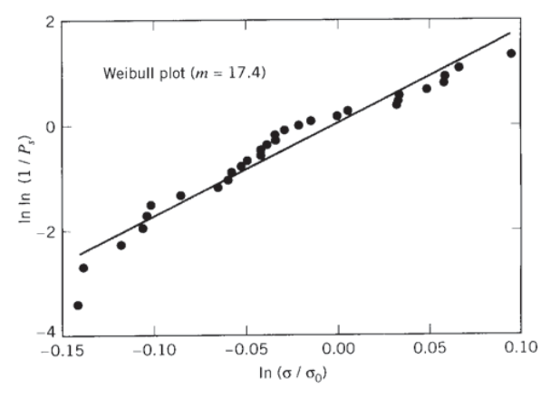
The Weibull plot of these data is shown in Figure 6; the regression slope is 17.4.
Similarly to the B-basis design allowable for the normal distribution, the B-allowable can also be computed from the Weibull parameters \(m\) and \(\sigma_0\). The procedure is(S.W. Rust, et al., ASTM STP 1003, p. 136, 1989. (Also Military Handbook 17.))
\(B = Q \exp [\dfrac{-V}{m\sqrt{N}}]\)
where \(Q\) and \(V\) are
\(Q = \sigma_0 (0.10536)^{1/m}\)
Example \(\PageIndex{7}\)
The B-allowable is computed for the 30-test population as
\(Q = 75.46 (0.10536)^{1/17.4m} = 66.30\)
\(B = 66.30 \exp [\dfrac{-5.03}{17.4\sqrt{30}}] = 62.89\)
This value is somewhat lower than the 65.05 obtained as the normal-distribution B-allowable, so in this case the Weibull method is a bit more lenient.
The Weibull equation can be used to predict the magnitude of the size effect. If for instance we take a reference volume \(V_0\) and express the volume of an arbitrary specimen as \(V = nV_0\), then the probability of failure at volume \(V\) is found by multiplying \(P_s(V)\) by itself \(n\) times:
\(P_s (V) = [P_s(V_0)]^n = [P_s(V_0)]^{V/V_0}\)
\[P_s(V) = \exp -\dfrac{V}{V_0} (\dfrac{\sigma}{\sigma_0})^m\]
Hence the probability of failure increases exponentially with the specimen volume. This is another danger in simple scaling, beyond the area vs. volume argument we outlined in Module 1.
Example \(\PageIndex{8}\)
Solving Equation 6.3.7, the stress for a given probability of survival is
\(\sigma= [\dfrac{-\ln (P_s)}{(V/V_0)}]^{\tfrac{1}{n}} \sigma_0\)
Using \(\sigma_0 = 75.46\) and \(n = 17.4\) for the 30-specimen population, the stress for \(P_s = .5\) and \(V/V_0 = 1\) is \(\sigma = 73.9\text{kpsi}\). If now the specimen size is doubled, so that \(V/V_0 = 2\), the probability of survival at this stress as given by Equation 6.3.7 drops to \(P_s = 0.25\). If on the other hand the specimen size is halved \((V/V_0 = 0.5)\), the probability of survival rises to \(P_s = 0.71\).
A final note of caution, a bit along the lines of the famous Mark Twain aphorism about there being "lies, damned lies, and statistics:" it is often true that populations of simple tensile or other laboratory specimens can be well described by classical statistical distributions. This should not be taken to imply that more complicated structures such as bridges and airplanes can be so neatly described. For instance, one aircraft study cited by Gordon(J.E. Gordon, Structures, Plenum Press, 1978.) found failures to occur randomly and uniformly over a wide range extending both above and below the statistically- based design safe load. Any real design, especially for structures that put human life at risk, must be checked in every reasonable way the engineer can imagine. This will include proof testing to failure, consideration of the worst possible environmental factors, consideration of construction errors resulting from difficult-to-manufacture designs, and so on almost without limit. Experience, caution and common sense will usually be at least as important as elaborate numerical calculations.
Exercise \(\PageIndex{1}\)
Ten strength measurements have produced a mean tensile strength of \(\overline{\sigma_f} = 100\) MPa, with 95% confidence limits of \(\pm 8\) MPa. How many additional measurements would be necessary to reduce the confidence limits by half, assuming the mean and standard deviation of the measurements remains unchanged?
Exercise \(\PageIndex{2}\)
The thirty measurements of the tensile strength of graphite/epoxy composite listed in Example \(\PageIndex{1}\) were made at room temperature. Thirty additional tests conducted at 93\(^{\circ} C\) gave the values (in kpsi): 63.40, 69.70, 72.80, 63.60, 71.20, 72.07, 76.97, 70.94, 76.22, 64.65, 62.08, 61.53, 70.53, 72.88, 74.90, 78.61, 68.72, 72.87, 64.49, 75.12, 67.80, 72.68, 75.09, 67.23, 64.80, 75.84, 63.87, 72.46, 69.54, 76.97. For these data:
- Determine the arithmetic mean, standard deviation, and coefficient of variation.
- Determine the 95% confidence limits on the mean strength.
- Determine whether the average strengths at 23\(^{\circ} C\) and 93\(^{\circ} C\) are statistically different.
- Determine the normal and Weibull B-allowable strengths.
- Plot the cumulative probability of failure \(P_f\) vs. the failure stress on normal probability paper.
- Do the data appear to be distributed normally, based on the \(\chi^2\) test?
- Plot the cumulative probability of survival \(P_s\) vs. the failure stress on Weibull probability paper.
- Determine the Weibull parameters \(\sigma_0\) and \(m\).
- Estimate how the mean strength would change if the specimens were made ten times smaller, or ten times larger.
Exercise \(\PageIndex{3}\)
Repeat the previous problem, but using data for -59◦C: 55.62, 55.91, 56.73, 57.54, 58.28, 59.23, 60.39, 60.62, 61.1, 62.1, 63.69, 63.8, 64.7, 65.2, 65.33, 66.39, 66.43, 66.72, 67.05, 67.76, 68.84, 69.15, 69.3, 69.37, 69.82, 70.94, 71.39, 71.74, 72.2, 73.46.
Appendix - Statistical Tables and Paper
Following are several standard tables and graph papers that can be used in performing statistical calculations, in the event suitable software is not available.
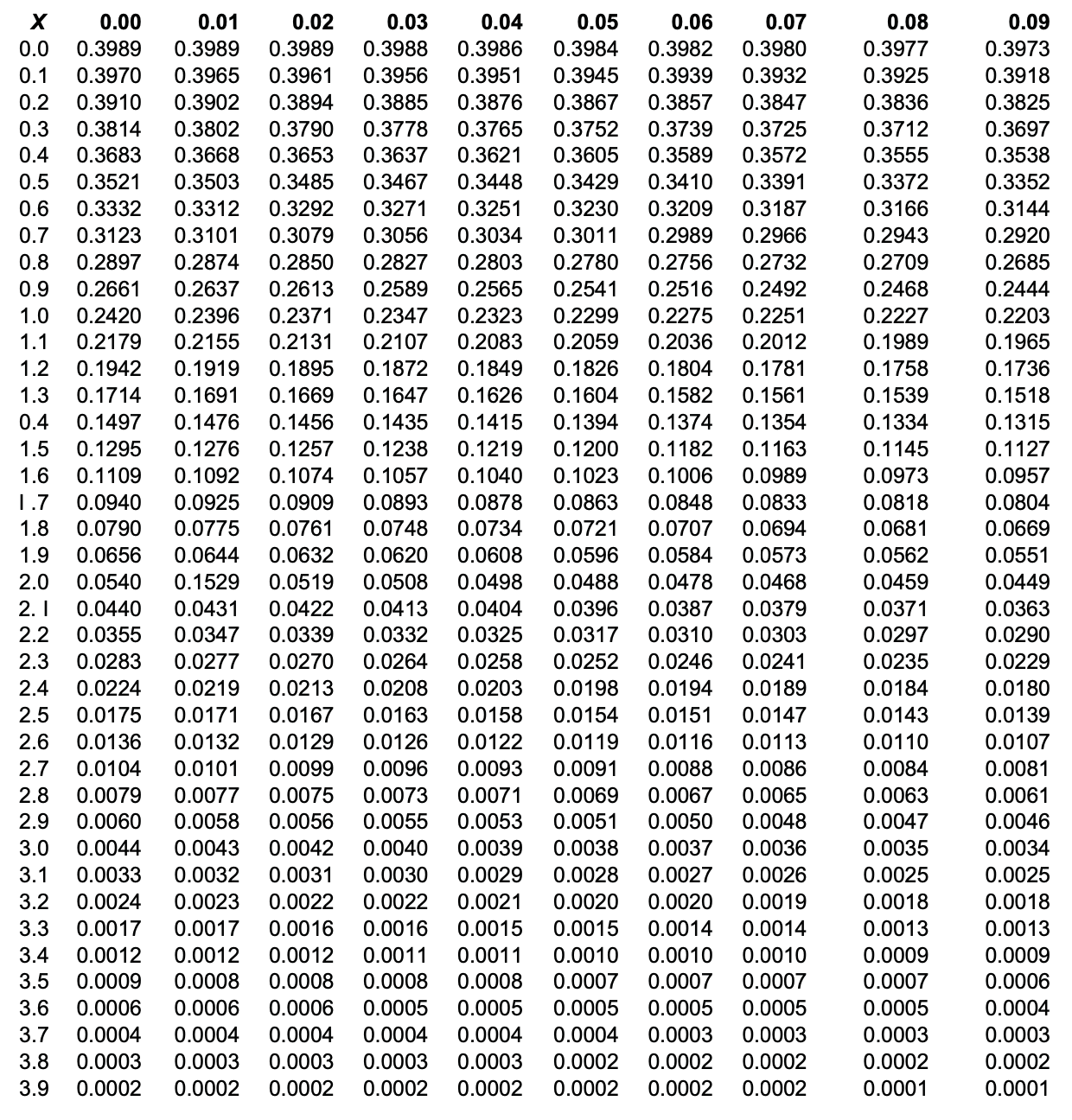
1. Normal Distribution Table
2. Cumulative Normal Distribution Table
3. Chi-Square Table
4. \(t\)-Distribution
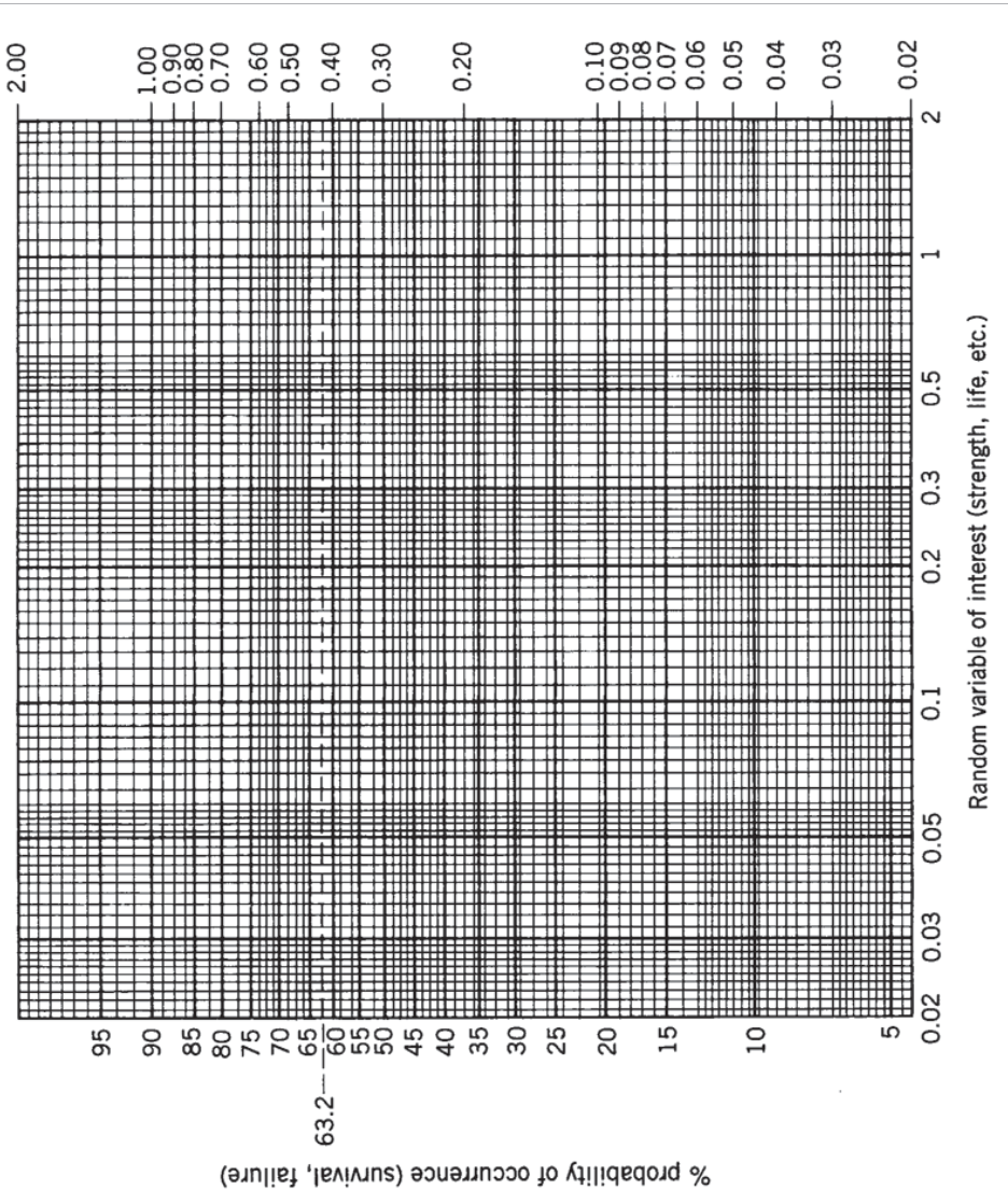
5. Normal Probability Paper
6. Weibull Paper
1. Normal Distribution
2. Cumulative Normal Distribution
4. \(t\)-Distribution
5. Normal Probability Paper
6. Weibull Paper