
6.4: Introduction to Fracture Mechanics
- Page ID
- 44553

Introduction
In 1983, the National Bureau of Standards (now the National Institute for Science and Technology) and Battelle Memorial Institute (R.P. Reed et al., NBS Special Publication 647-1, Washington, 1983.) estimated the costs for failure due to fracture to be $119 billion per year in 1982 dollars. The dollars are important, but the cost of many failures in human life and injury is infinitely more so.
Failures have occurred for many reasons, including uncertainties in the loading or environment, defects in the materials, inadequacies in design, and deficiencies in construction or maintenance. Design against fracture has a technology of its own, and this is a very active area of current research. This module will provide an introduction to an important aspect of this field, since without an understanding of fracture the methods in stress analysis discussed previously would be of little use. We will focus on fractures due to simple tensile overstress, but the designer is cautioned again about the need to consider absolutely as many factors as possible that might lead to failure, especially when life is at risk.
The Module on the Dislocation Basis of Yield (Module 21) shows how the strength of structural metals – particularly steel – can be increased to very high levels by manipulating the microstructure so as to inhibit dislocation motion. Unfortunately, this renders the material in- creasingly brittle, so that cracks can form and propagate catastrophically with very little warn- ing. An unfortunate number of engineering disasters are related directly to this phenomenon, and engineers involved in structural design must be aware of the procedures now available to safeguard against brittle fracture.
The central difficulty in designing against fracture in high-strength materials is that the presence of cracks can modify the local stresses to such an extent that the elastic stress analyses done so carefully by the designers are insufficient. When a crack reaches a certain critical length, it can propagate catastrophically through the structure, even though the gross stress is much less than would normally cause yield or failure in a tensile specimen. The term “fracture mechanics” refers to a vital specialization within solid mechanics in which the presence of a crack is assumed, and we wish to find quantitative relations between the crack length, the material’s inherent resistance to crack growth, and the stress at which the crack propagates at high speed to cause structural failure.
The energy-balance approach
When A.A. Griffith (1893–1963) began his pioneering studies of fracture in glass in the years just prior to 1920, he was aware of Inglis’ work in calculating the stress concentrations around elliptical holes, and naturally considered how it might be used in developing a fundamental approach to predicting fracture strengths. However, the Inglis solution poses a mathematical difficulty: in the limit of a perfectly sharp crack, the stresses approach infinity at the crack tip. This is obviously nonphysical (actually the material generally undergoes some local yielding to blunt the cracktip), and using such a result would predict that materials would have near-zero strength: even for very small applied loads, the stresses near crack tips would become infinite, and the bonds there would rupture. Rather than focusing on the crack-tip stresses directly, Griffith employed an energy-balance approach that has become one of the most famous developments in materials science(A.A. Griffith, Philosophical Transactions, Series A, Vol. 221, pp. 163–198, 1920. The importance of Griffith’s work in fracture was largely unrecognized until the 1950’s. See J.E. Gordon, The Science of Structures and Materials, Scientific American Library, 1988, for a personal account of the Griffith story.).
The strain energy per unit volume of stressed material is
\(U^* = \dfrac{1}{V} \int f\ dx = \int \dfrac{f}{A} \dfrac{dx}{L} =\int \sigma d\epsilon\)
If the material is linear (\(\sigma = E_{\epsilon}\)), then the strain energy per unit volume is
\(U^* = \dfrac{E_{\epsilon}^2}{2} = \dfrac{\sigma^2}{2E}\)
When a crack has grown into a solid to a depth \(a\), a region of material adjacent to the free surfaces is unloaded, and its strain energy released. Using the Inglis solution, Griffith was able to compute just how much energy this is.
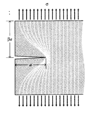
A simple way of visualizing this energy release, illustrated in Figure 1, is to regard two triangular regions near the crack flanks, of width \(a\) and height \(\beta_a\), as being completely unloaded, while the remaining material continues to feel the full stress \(\sigma\). The parameter \(\beta\) can be selected so as to agree with the Inglis solution, and it turns out that for plane stress loading \(\beta = \pi\). The total strain energy \(U\) released is then the strain energy per unit volume times the volume in both triangular regions:
\(U = -\dfrac{\sigma^2}{2E} \cdot \pi a^2\)
Here the dimension normal to the \(x-y\) plane is taken to be unity, so \(U\) is the strain energy released per unit thickness of specimen. This strain energy is liberated by crack growth. But in forming the crack, bonds must be broken, and the requisite bond energy is in effect absorbed by the material. The surface energy \(S\) associated with a crack of length \(a\) (and unit depth) is:
\(S = 2 \gamma a\)
where \(\gamma\) is the surface energy (e.g., Joules/meter\(^2\)) and the factor 2 is needed since two free surfaces have been formed. As shown in Figure 2, the total energy associated with the crack is then the sum of the (positive) energy absorbed to create the new surfaces, plus the (negative) strain energy liberated by allowing the regions near the crack flanks to become unloaded.
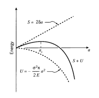
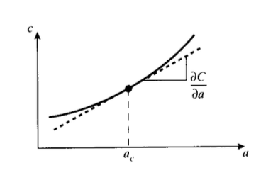
As the crack grows longer (\(a\) increases), the quadratic dependence of strain energy on a eventually dominates the surface energy, and beyond a critical crack length ac the system can lower its energy by letting the crack grow still longer. Up to the point where \(a = a_c\), the crack will grow only if the stress in increased. Beyond that point, crack growth is spontaneous and catastrophic.
The value of the critical crack length can be found by setting the derivative of the total energy \(S+U\) to zero:
Since fast fracture is imminent when this condition is satisfied, we write the stress as \(\sigma_f\). Solving,
\(\sigma_f = \sqrt{\dfrac{2E_{\gamma}}{\pi a}}\)
Griffith's original work dealt with very brittle materials, specifically glass rods. When the material exhibits more ductility, consideration of the surface energy alone fails to provide an accurate model for fracture. This deficiency was later remedied, at least in part, independently by Irwin(G.R. Irwin, "Fracture Dynamics," Fracturing of Metals, American Society for Metals, Cleveland, 1948.) and Orowan(E. Orowan, "Fracture and Strength of Solids," Report of Progress in Physics, Vol. 12, 1949.). They suggested that in a ductile material a good deal – in fact the vast majority – of the released strain energy was absorbed not by creating new surfaces, but by energy dissipation due to plastic flow in the material near the crack tip. They suggested that catastrophic fracture occurs when the strain energy is released at a rate sufficient to satisfy the needs of all these energy "sinks," and denoted this critical strain energy release rate by the parameter \(\mathcal{G}_c\); the Griffith equation can then be rewritten in the form:
\[\sigma_f = \sqrt{\dfrac{E\mathcal{G}_c}{\pi a}}\]
This expression describes, in a very succinct way, the interrelation between three important aspects of the fracture process: the material, as evidenced in the critical strain energy release rate \(\mathcal{G}_c\); the stress level \(\sigma_f\); and the size, \(a\), of the flaw. In a design situation, one might choose a value of a based on the smallest crack that could be easily detected. Then for a given material with its associated value of \(\mathcal{G}_c\), the safe level of stress \(\sigma_f\) could be determined. The structure would then be sized so as to keep the working stress comfortably below this critical value.
Example \(\PageIndex{1}\)
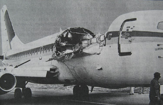
The story of the DeHavilland Comet aircraft of the early 1950’s, in which at least two aircraft disintegrated in flight, provides a tragic but fascinating insight into the importance of fracture theory. It is an eerie story as well, having been all but predicted in a 1948 novel by Nevil Shute named No Highway. The book later became a movie starring James Stewart as a perserverant metallurgist convinced that his company’s new aircraft (the “Reindeer”) was fatally prone to metal fatigue. When just a few years later the Comet was determined to have almost exactly this problem, both the book and the movie became rather famous in the materials engineering community.
The postmortem study of the Comet’s problems was one of the most extensive in engineering history(T. Bishop, Metal Progress, Vol. 67, pp. 79–85, May 1955.). It required salvaging almost the entire aircraft from scattered wreckage on the ocean floor and also involved full-scale pressurization of an aircraft in a giant water tank. Although valuable lessons were learned, it is hard to overstate the damage done to the DeHavilland Company and to the British aircraft industry in general. It is sometimes argued that the long predominance of the United States in commercial aircraft is due at least in part to the Comet’s misfortune.
The Comet aircraft had a fuselage of clad aluminum, with \(\mathcal{G}_c \approx 300\) in-psi. The hoop stress due to relative cabin pressurization was 20,000 psi, and at that stress the length of crack that will propagate catastrophically is
\[a = \dfrac{\mathcal{G}_c E}{\pi \sigma^2} = \dfrac{(300)(11 \times 10^6)}{\pi (20 \times 10^3)^2} = 2.62'' \nonumber\]
A crack would presumably be detected in routine inspection long before it could grow to this length. But in the case of the Comet, the cracks were propagating from rivet holes near the cabin windows. When the crack reached the window, the size of the window opening was effectively added to the crack length, leading to disaster.
Modern aircraft are built with this failure mode in mind, and have "tear strips" that are supposedly able to stop any rapidly growing crack. But this remedy is not always effective, as was demonstrated in 1988 when a B737 operated by Aloha Airlines had the roof of the first-class cabin tear away. That aircraft had stress-corrosion damage at a number of rivets in the fuselage lap splices, and this permitted multiple small cracks to link up to form a large crack. A great deal of attention is currently being directed to protection against this sort of "multi-site damage."
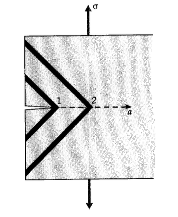
It is important to realize that the critical crack length is an absolute number, not depending on the size of the structure containing it. Each time the crack jumps ahead, say by a small increment \(\delta a\), an additional quantity of strain energy is released from the newly-unloaded material near the crack. Again using our simplistic picture of a triangular-shaped region that is at zero stress while the rest of the structure continues to feel the overall applied stress, it is easy to see in Figure 3 that much more more energy is released due to the jump at position 2 than at position 1. This is yet another reason why small things tend to be stronger: they simply aren’t large enough to contain a critical-length crack.
Example \(\PageIndex{2}\)
Gordon (J.E. Gordon, Structures, or Why Things Don’t Fall Down, Plenum, New York, 1978.) tells of a ship’s cook who one day noticed a crack in the steel deck of his galley. His superiors assured him that it was nothing to worry about — the crack was certainly small compared with the vast bulk of the ship — but the cook began painting dates on the floor to mark the new length of the crack each time a bout of rough weather would cause it to grow longer. With each advance of the crack, additional decking material was unloaded, and the strain energy formerly contained in it released. But as the amount of energy released grows quadratically with the crack length, eventually enough was available to keep the crack growing even with no further increase in the gross load. When this happened, the ship broke into two pieces; this seems amazing but there are a more than a few such occurrences that are very well documented. As it happened, the part of the ship with the marks showing the crack’s growth was salvaged, and this has become one of the very best documented examples of slow crack growth followed by final catastrophic fracture.
Compliance calibration
A number of means are available by which the material property \(\mathcal{G}_c\) can be measured. One of these is known as compliance calibration, which employs the concept of compliance as a ratio of deformation to applied load: \(C = \delta/P\). The total strain energy \(U\) can be written in terms of this compliance as:
\(U = \dfrac{1}{2} P \delta = \dfrac{1}{2} CP^2\)
The compliance of a suitable specimen, for instance a cantilevered beam, could be measured experimentally as a function of the length a of a crack that is grown into the specimen (see Figure 4. The strain energy release rate can then be determined by differentiating the curve of compliance versus length:
\[\mathcal{G} = \dfrac{\partial U}{\partial a} = \dfrac{1}{2} P^2 \dfrac{\partial C}{\partial a}\]
The critical value of \(\mathcal{G}\), \(\mathcal{G}_c\), is then found by measuring the critical load \(P_c\) needed to fracture a specimen containing a crack of length \(a_c\), and using the slope of the compliance curve at this same value of \(a\):
\[\mathcal{G}_c = \dfrac{1}{2}P_c^2 \dfrac{\partial C}{\partial a} |_{a = a_c}\]
Example \(\PageIndex{3}\)
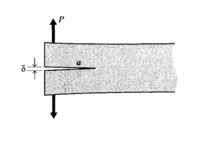
For a double-cantilever beam (DCB) specimen such as that shown in Figure 5, beam theory gives the deflection as
\(\dfrac{\delta}{2} = \dfrac{Pa^3}{3EI}\)
where \(I = bh^3/12\). The elastic compliance is then
\(C = \dfrac{\delta}{P} = \dfrac{2a^3}{3EI}\)
If the crack is observed to jump forward when \(P = P_c\), Equation 3 can be used to compute the critical strain energy release rate as
\(\mathcal{G}_c = \dfrac{1}{2} P_c^2 \cdot \dfrac{2a^3}{EI} = \dfrac{12P_c^2 a^2}{b^2h^3E}\)
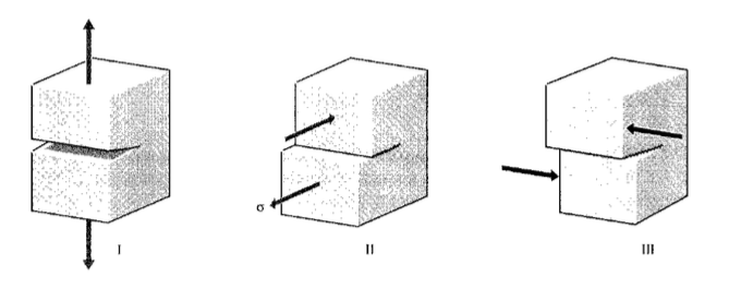
The stress intensity approach
While the energy-balance approach provides a great deal of insight to the fracture process, an alternative method that examines the stress state near the tip of a sharp crack directly has proven more useful in engineering practice. The literature treats three types of cracks, termed mode I, II, and III as illustrated in Figure 6. Mode I is a normal-opening mode and is the one we shall emphasize here, while modes II and III are shear sliding modes. As was outlined in Module 16, the semi-inverse method developed by Westergaard shows the opening-mode stresses to be:
\[\begin{array} {c} {\sigma_x = \dfrac{K_I}{\sqrt{2\pi r}} \cos \dfrac{\theta}{2} (1 - \sin \dfrac{\theta}{2} \sin \dfrac{3 \theta}{2}) + \dots} \\ {\sigma_y = \dfrac{K_I}{\sqrt{2\pi r}} \cos \dfrac{\theta}{2} (1 + \sin \dfrac{\theta}{2} \sin \dfrac{3 \theta}{2}) + \dots} \\ {\tau_{xy} = \dfrac{K_I}{\sqrt{2\pi r}} \cos \dfrac{\theta}{2} \cos \dfrac{3\theta}{2} \sin \dfrac{\theta}{2} \cdots} \end{array}\]
For distances close to the crack tip \((r\le 0.1a)\), the second and higher order terms indicated by dots may be neglected. At large distances from the crack tip, these relations cease to apply and the stresses approach their far-field values that would obtain were the crack not present.
The \(KI\) in Eqns. 6.4.4 is a very important parameter known as the stress intensity factor. The I subscript is used to denote the crack opening mode, but similar relations apply in modes II and III. The equations show three factors that taken together depict the stress state near the crack tip: the denominator factor \((2\pi r)^{-1/2}\) shows the singular nature of the stress distribution; \(\sigma\) approaches infinity as the crack tip is approached, with a \(r^{-1/2}\) dependency. The angular dependence is separable as another factor: e.g. \(f_x = \cos \theta/2 \cdot (1 - \sin \theta/2 \sin 3\theta/2) + \cdots\). The factor \(K_I\) contains the dependence on applied stress \(\sigma_{\infty}\), the crack length \(a\), and the specimen geometry. The \(KI\) factor gives the overall intensity of the stress distribution, hence its name.
For the specific case of a central crack of width \(2a\) or an edge crack of length \(2a\) in a large sheet, \(K_I = \sigma_{\infty} \sqrt{\pi a}\), and \(K_I = 1.12 \sigma_{\infty} \sqrt{\pi a}\) for an edge crack of length \(2a\) in a large sheet. (The factor \(\pi\) could obviously be canceled with the \(\pi\) in the denominator of Equation 6.4.4, but is commonly retained for consistency with earlier work.) Expressions for \(K_I\) for some additional geometries are given in Table 1. The literature contains expressions for \(K\) for a large number of crack and loading geometries, and both numerical and experimental procedures exist for determining the stress intensity factor is specific actual geometries.
| Type of Crack | Stress Intensity Factor, \(K_I\) |
| Center crack, length \(2a\), in an infinite plate | \(\sigma_{\infty} \sqrt{\pi a}\) |
| Edge crack, length \(a\), in a semi-infinite plate | \(1.12 \sigma_{\infty} \sqrt{\pi a}\) |
| Central penny-shaped crack, radius \(a\), in infinite body | \(2 \sigma_{\infty} \sqrt{\tfrac{a}{\pi}}\) |
| Center crack, length \(2a\) in plate of width \(W\) | \(\sigma_{\infty} \sqrt{W \tan (\tfrac{\pi a}{W})}\) |
| 2 symmetrical edge cracks, each length \(a\), in plate of total width \(W\) | \(\sigma_{\infty} \sqrt{W[\tan (\tfrac{\pi a}{W}) + 0.1 \sin (\dfrac{2 \pi a}{W})]}\) |
These stress intensity factors are used in design and analysis by arguing that the material can withstand crack tip stresses up to a critical value of stress intensity, termed \(K_{Ic}\), beyond which the crack propagates rapidly. This critical stress intensity factor is then a measure of material toughness. The failure stress \(\sigma_f\) is then related to the crack length a and the fracture toughness by
\[\sigma_f = \dfrac{K_{Ic}}{\alpha \sqrt{\pi a}}\]
where \(\alpha\) is a geometrical parameter equal to 1 for edge cracks and generally on the order of unity for other situations. Expressions for α are tabulated for a wide variety of specimen and crack geometries, and specialty finite element methods are available to compute it for new situations.
The stress intensity and energy viewpoints are interrelated, as can be seen by comparing Eqns. 6.4.1 and 6.4.5 (with \(\alpha = 1\)):
\(\sigma_f = \sqrt{\dfrac{E\mathcal{G}_c}{\pi a}} = \dfrac{K_{Ic}}{\sqrt{\pi a}} \to K_{Ic}^2 = E \mathcal{G}_c\)
This relation applies in plane stress; it is slightly different in plane strain:
For metals with \(v = .3\), \((1 - v^2) = 0.91\). This is not a big change; however, the numerical values of \(\mathcal{G}_c\) or \(K_{Ic}\) are very different in plane stress or plane strain situations, as will be described below.
Typical values of \(G_{Ic}\) and \(K_{Ic}\) for various materials are listed in Table 2, and it is seen that they vary over a very wide range from material to material. Some polymers can be very tough, especially when rated on a per-pound bases, but steel alloys are hard to beat in terms of absolute resistance to crack propagation.
| Material | \(G_{Ic} (kJm^{-2})\) | \(K_{Ic}(MNm^2)\) | \(E(GPa)\) |
|---|---|---|---|
| Steel alloy | 107 | 150 | 210 |
| Aluminum alloy | 20 | 37 | 69 |
| Polyethylene | 20 (\(J_{Ic}\)) | - | 0.15 |
| High-impact polystyrene | 15.8 (\(J_{Ic}\)) | - | 2.1 |
| Steel - mild | 12 | 50 | 210 |
| Rubber | 13 | - | 0.001 |
| Glass-reinforced thermoset | 7 | 7 | 7 |
| Rubber-toughened epoxy | 2 | 2.2 | 2.4 |
| PMMA | 0.5 | 1.1 | 2.5 |
| Polystyrene | 0.4 | 1.1 | 3 |
| Wood | 0.12 | 0.5 | 2.1 |
| Glass | 0.007 | 0.7 | 70 |
Example \(\PageIndex{4}\)
Equation 6.4.5 provides a design relation among the applied stress \(\sigma\), the material’s toughness \(K_{Ic}\), and the crack length \(a\). Any one of these parameters can be calculated once the other two are known. To illustrate one application of the process, say we wish to determine the safe operating pressure in an aluminum pressure vessel 0.25 m in diameter and with a 5 mm wall thickness. First assuming failure by yield when the hoop stress reaches the yield stress (330 MPa) and using a safety factor of 0.75, we can compute the maximum pressure as
\(p = \dfrac{0.75 \sigma t}{r} = \dfrac{0.75 \times 330 \times 10^6}{0.25/2} = 9.9\text{ MPa} = 1400\text{ psi}\)
To insure against failure by rapid crack growth, we now calculate the maximum crack length permissible at the operating stress, using a toughness value of \(K_{Ic} = 41 \text{ MPa} \sqrt{m}\):
\(a = \dfrac{K_{Ic}^2}{\pi \sigma^2} = \dfrac{(41 \times 10^6)^2}{\pi (0.75 \times 330 \times 10^6)^2} = 0.01\ m = 0.4\ in\)
Here an edge crack with \(\alpha = 1\) has been assumed. An inspection schedule must be implemented that is capable of detecting cracks before they reach this size.
Effect of specimen geometry
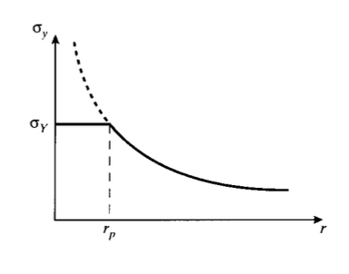
The toughness, or resistance to crack growth, of a material is governed by the energy absorbed as the crack moves forward. In an extremely brittle material such as window glass, this energy is primarily just that of rupturing the chemical bonds along the crack plane. But as already mentioned, in tougher materials bond rupture plays a relatively small role in resisting crack growth, with by far the largest part of the fracture energy being associated with plastic flow near the crack tip. A "plastic zone" is present near the crack tip within which the stresses as predicted by Equation 6.4.4 would be above the material’s yield stress \(\sigma_Y\). Since the stress cannot rise above \(\sigma_Y\), the stress in this zone is \(\sigma_Y\) rather than that given by Equation 6.4.4. To a first approximation, the distance rp this zone extends along the \(x\)-axis can be found by using Equation 6.4.4 with \(\theta = 0\) to find the distance at which the crack tip stress reduces to \(\sigma_Y\):
\(\sigma_y = \sigma_Y = \dfrac{K_I}{\sqrt{2\pi r_p}}\)
\[r_p = \dfrac{K_I^2}{2 \pi \sigma_Y^2\]
This relation is illustrated in Figure 7. As the stress intensity in increased either by raising the imposed stress or by crack lengthening, the plastic zone size will increase as well. But the extent of plastic flow is ultimately limited by the material’s molecular or microstructural mobility, and the zone can become only so large. When the zone can grow no larger, the crack can no longer be constrained and unstable propagation ensues. The value of \(K_I\) at which this occurs can then be considered a materials property, named \(K_{Ic}\).
In order for the measured value of \(K_{Ic}\) to be valid, the plastic zone size should not be so large as to interact with the specimen’s free boundaries or to destroy the basic nature of the singular stress distribution. The ASTM specification for fracture toughness testing(E 399-83, "Standard Test Method for Plane-Strain Fracture Toughness of Metallic Materials," ASTM, 1983.) specifies the specimen geometry to insure that the specimen is large compared to the crack length and the plastic zone size (see Figure 8):
Figure 8: Dimensions of fracture toughness specimen.
A great deal of attention has been paid to the important case in which enough ductility exists to make it impossible to satisfy the above criteria. In these cases the stress intensity view must be abandoned and alternative techniques such as the J-integral or the crack tip opening displacement method used instead. The reader is referred to the references listed at the end of the module for discussion of these approaches.
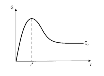
The fracture toughness as measured by \(K_c\) or \(\mathcal{G}_c\) is essentially a measure of the extent of plastic deformation associated with crack extension. The quantity of plastic flow would be expected to scale linearly with the specimen thickness, since reducing the thickness by half would naturally cut the volume of plastically deformed material approximately in half as well. The toughness therefore rises linearly, at least initially, with the specimen thickness as seen in Figure 9. Eventually, however, the toughness is observed to go through a maximum and fall thereafter to a lower value. This loss of toughness beyond a certain critical thickness \(t^*\) is extremely important in design against fracture, since using too thin a specimen in measuring toughness will yield an unrealistically optimistic value for \(\mathcal{G}_C\). The specimen size requirements for valid fracture toughness testing are such that the most conservative value is measured.
The critical thickness is that which causes the specimen to be dominated by a state of plane strain, as opposed to plane stress. The stress in the through-thickness \(z\) direction must become zero at the sides of the specimen since no traction is applied there, and in a thin specimen the stress will not have room to rise to appreciable values within the material. The strain in the \(z\) direction is not zero, of course, and the specimen will experience a Poisson contraction given by \(\epsilon_z = v(\sigma_x + \sigma_y)\). But when the specimen is thicker, material near the center will be unable to contract laterally due to the constraint of adjacent material. Now the \(z\)-direction strain is zero, so a tensile stress will arise as the material tries to contract but is prevented from doing so. The value of σz rises from zero at the outer surface and approaches a maximum value given by \(\sigma_z \approx v(\sigma_x + \sigma_y)\) in a distance \(t^*\) as seen in Figure 10. To guarantee that plane strain conditions dominate, the specimen thickness \(t\) must be such that \(t \gg 2t^*\).
The triaxial stress state set up near the center of a thick specimen near the crack tip reduces the maximum shear stress available to drive plastic flow, since the maximum shear stress is equal to one half the difference of the largest and smallest principal stress, and the smallest is now greater than zero. Or equivalently, we can state that the mobility of the material is constrained by the inability to contract laterally. From either a stress or a strain viewpoint, the extent of available plasticity is reduced by making the specimen thick.
Example \(\PageIndex{5}\)
The plastic zone sizes for the plane stress and plane strain cases can be visualized by using a suitable yield criterion along with the expressions for stress near the crack tip. The v. Mises yield criterion was given in terms of principal stresses in Module 20 as
The principal stresses can be obtained from Eqns. 6.4.4 as
\(\sigma_1 = \dfrac{K_I}{\sqrt{2 \pi r}} \cos \dfrac{\theta}{2} (1 + \sin \dfrac{\theta}{2})\)
The third principal stress is
\(\sigma_3 = \begin{cases} 0, \text{ plane stress} \\ v(\sigma_1 + \sigma_2), \text{ plane strain} \end{cases}\)
These stresses can be substituted into the yield criterion, which is then solved for the radius \(r\) at which yield occurs. It is convenient to normalize this radius by the raduis of the plastic zone along the \(x\)−axis, given by Equation 6.4.6. Maple commands to carry out these substitutions and plot the result are:
# Radius of plastic zone along x-axis > rp:=K[I]^2/(2*Pi*sigma[Y]^2):
# v. Mises yield criterion in terms of principal stresses
> v_mises:=2*sigma[Y]^2= (sigma[1]-sigma[2])^2 + (sigma[1]-sigma[3])^2 + (sigma[2]-sigma[3])^2:
# Principal stresses in crack-tip region
> sigma[1]:=(K[I]/sqrt(2*Pi*r))*cos(theta/2)*(1+sin(theta/2)):
> sigma[2]:=(K[I]/sqrt(2*Pi*r))*cos(theta/2)*(1-sin(theta/2));
# Evaluate v. Mises for plane stress (v_strs) and plane strain (v_strn) # Take nu = 0.3
> v_strs:=subs(sigma[3]=0,v_mises):
> v_strn:=subs(sigma[3]=.3*(sigma[1]+sigma[2]),v_mises):
# Solve for plastic zone radius, normalize by rp
# pl_strs for plane stress case, pl_strn for plane strain > pl_strs:=solve(v_strs,r)/rp:
> pl_strn:=solve(v_strn,r)/rp:
# Plot normalized plastic zones for plane stress and plane strain > plot({pl_strs,pl_strn},theta=0..2*Pi,coords=polar);
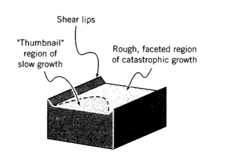
Even in a thick specimen, the z-direction stress must approach zero at the side surfaces. Regions near the surface are therefore free of the triaxial stress constraint, and exhibit greater shear-driven plastic flow. After a cracked specimen has been tested to failure, a flat “thumbnail” pattern will often be visible as illustrated in Figure 12. This is the region of slow crack growth, where the crack is able to maintain its preferred orientation transverse to the y-direction stress. The crack growth near the edges is retarded by the additional plastic flow there, so the crack line bows inward. When the stress is increased enough to cause the crack to grow catastrophically, it typically does so at speeds high enough that the transverse orientation is not always maintained. The region of rapid fracture is thus faceted and rough, leading some backyard mechanics to claim the material failed because it "crystallized."
Along the edges of the specimen, "shear lips" can often be found on which the crack has developed by shear flow and with intensive plastic deformation. The lips will be near a 45\(^{\circ}\) angle, the orientation of the maximum shear planes.
Grain size and temperature
Steel is such an important and widely used structural material that it is easy to forget that steel is a fairly recent technological innovation. Well into the nineteenth century, wood was the dominant material for many bridges, buildings, and ships. As the use of iron and steel became more widespread in the latter part of that century and the first part of the present one, a number of disasters took place that can be traced to the then-incomplete state of understanding of these materials, especially concerning their tendency to become brittle at low temperatures. Many of these failures have been described and analyzed in a fascinating book by Parker(E.R. Parker, Brittle Behavior of Engineering Structures, John Wiley & Sons, 1957.).
One of these brittle failures is perhaps the most famous disaster of the last several centuries, the sinking of the transatlantic ocean liner Titanic on April 15, 1912, with a loss of some 1,500 people and only 705 survivors. Until very recently, the tragedy was thought to be caused by a long gash torn through the ship’s hull by an iceberg. However, when the wreckage of the ship was finally discovered in 1985 using undersea robots, no evidence of such a gash was found. Further, the robots were later able to return samples of the ship’s steel whose analysis has given rise to an alternative explanation.
It is now well known that lesser grades of steel, especially those having large concentrations of impurities such as interstitial carbon inclusions, are subject to embrittlement at low temperatures. William Garzke, a naval architect with the New York firm of Gibbs & Cox, and his colleagues have argued that the steel in the Titanic was indeed brittle in the 31\(^{\circ}F\) waters of the Atlantic that night, and that the 22-knot collision with the iceberg generated not a gash but extensive cracking through which water could enter the hull. Had the steel remained tough at this temperature, these authors feel, the cracking may have been much less extensive. This would have slowed the flooding and allowed more time for rescue vessels to reach the scene, which could have increased greatly the number of survivors.
In the bcc transition metals such as iron and carbon steel, brittle failure can be initiated by dislocation glide within a crystalline grain. The slip takes place at the yield stress \(\sigma_Y\), which varies with grain size according to the Hall-Petch law as described in Module 21:
\(\sigma_Y = \sigma_0 + k_Y d^{-1/2}\)
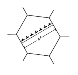
Dislocations are not able to propagate beyond the boundaries of the grain, since adjoining grains will not in general have their slip planes suitably oriented. The dislocations then "pile up" against the grain boundaries as illustrated in Figure 13. The dislocation pileup acts similarly to an internal crack with a length that scales with the grain size d, intensifying the stress in the surrounding grains. Replacing a by \(d\) in the modified Griffith equation (Equation 6.4.1), the applied stress needed to cause fracture in adjacent grains is related to the grain size as
\(\sigma_f = k_f d^{-1/2}, k_f \propto \sqrt{\dfrac{E\mathcal{G}_c}{\pi}}\)
The above two relations for yielding and fracture are plotted in Figure 14 against inverse root grain size (so grain size increases to the left), with the slopes being \(k_Y\) and \(k_f\) respectively. When \(k_f > k_Y\), fracture will not occur until \(\sigma = \sigma_Y\) for values of d to the left of point \(A\), since yielding and slip is a prerequisite for cleavage. In this region the yielding and fracture stresses are the same, and the failure appears brittle since large-scale yielding will not have a chance to occur. To the right of point \(A\), yielding takes place prior to fracture and the material appears ductile. The point \(A\) therefore defines a critical grain size \(d^*\) at which a "nil-ductility" transition from ductile (grains smaller than \(d^*\)) to brittle failure will take place.
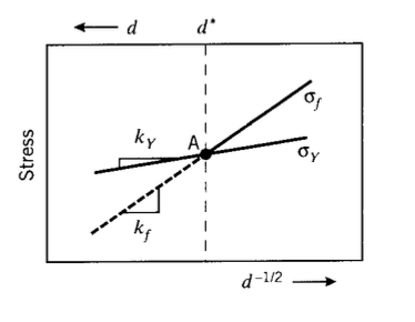
As the temperature is lowered, the yield stress σY will increase as described in Module 20, and the fracture stress σf will decrease (since atomic mobility and thus \(\mathcal{G}_C\) decrease). Therefore, point \(A\) shifts to the right as temperature is lowered. The critical grain size for nil ductility now occurs at a smaller value; i.e. the grains must be smaller to avoid embrittling the material. Equivalently, refining the grain size has the effect of lowering the ductile-brittle transition temperature. Hence grain-size refinement raises both the yield and fracture stress, lowers the ductile-brittle transition temperature, and promotes toughness as well. This is a singularly useful strengthening mechanism, since other techniques such as strain hardening and solid-solution hardening tend to achieve strengthening at the expense of toughness.
Factors other than temperature can also embrittle steel. Inclusions such as carbon and phosphorus act to immobilize slip systems that might otherwise relieve the stresses associated with dislocation pileups, and these inclusions can raise the yield stress and thus the ductile-brittle transition temperature markedly. Similar effects can be induced by damage from high-energy radiation, so embrittlement of nuclear reactor components is of great concern. Embrittlement is also facilitated by the presence of notches, since they generate triaxial stresses that constrain plastic flow. High strain rates promote brittleness because the flow stress needed to accommodate the strain rate is higher, and improper welding can lead to brittleness both by altering the steel’s microstructure and by generating residual internal stresses.
General References
- Anderson, T.L., Fracture Mechanics: Fundamentals and Applications, CRC Press, Boca Raton, 1991.
- Barsom, J.M., ed., Fracture Mechanics Retrospective, American Society for Testing and Materials, Philadelphia, 1987.
- Collins, J.A., Failure of Materials in Mechanical Design, Wiley, 1981.
- Courtney, T.H., Mechanical Behavior of Materials, McGraw-Hill, New York, 1990.
- Gordon, J.E., The New Science of Strong Materials, or Why You Don’t Fall Through the Floor, Princeton University Press, 1976.
- Hertzberg, R.W., Deformation and Fracture Mechanics of Engineering Materials, Wiley, New York, 1976.
- Knott, J.F., Fundamentals of Fracture Mechanics, John Wiley – Halsted Press, New York, 1973.
- Mendenhall, W., R.L. Scheaffer and D.D. Wackerly, Mathematical Statistics with Applica- tions, Duxbury Press, Boston, 1986.
- Strawley, J.E., and W.F. Brown, Fracture Toughness Testing, ASTM STP 381, 133, 1965.
- 1967.
Exercise \(\PageIndex{1}\)
Using a development analogous to that employed in Module 21 for the theoretical yield stress, show that the theoretical ultimate tensile strength is \(\sigma^{th} \approx E/10\) (much larger than that observed experimentally). Assume a harmonic atomic force function \(\sigma = \sigma^{th} \sin(2\pi x/\lambda\)), where \(x\) is the displacement of an atom from its equilibrium position and \(\lambda \approx a_0\) is the interatomic spacing. The maximum stress \(\sigma^{th}\) can then be found by using
\(E = (\dfrac{d \sigma}{d\epsilon})_{x \to 0} \text{ and } \epsilon = \dfrac{x}{a_0}\)
Exercise \(\PageIndex{2}\)
Using a safety factor of 2, find the safe operating pressure in a closed-end steel pressure vessel \(1'\) in diameter and \(0.2''\) wall thickness.
Exercise \(\PageIndex{3}\)
A pressure vessel is constructed with a diameter of \(d = 18''\) and a length of \(L = 6'\). The vessel is to be capable of withstanding an internal pressure of \(p = 1000\text{ psi}\), and the wall thickness is such as to keep the nominal hoop stress under \(2500\text{ psi}\). However, the vessel bursts at an internal pressure of only \(500\text{ psi}\), and a micrographic investigation reveals the fracture to have been initiated by an internal crack \(0.1''\) in length. Calculate the fracture toughness (\(K_{Ic}\)) of the material.
Exercise \(\PageIndex{4}\)
A highly cross-linked epoxy resin has a coefficient of linear thermal expansion \(\alpha = 5 \times 10^{-5} K^{-1}\), \(G_{IC} = 120 J/m^2\), \(E = 3.2 GPa\), and \(v = 0.35\). A thick layer of resin is cured and is firmly bonded to an aluminum part (\(\alpha = 2.5 \times 10^{-5} K^{-1}\)) at \(180^{\circ} C\). Calculate the minimum defect size needed to initiate cracking in the resin on cooling to \(20^{\circ} C\). Take \(\alpha\) in Equation 6.4.5 to be \(2/\pi\) for penny-shaped cracks of radius \(a\) in a wide sheet.
Exercise \(\PageIndex{5}\)
(a) A thick plate of aluminum alloy, 175 mm wide, contains a centrally-located crack 75 mm in length. The plate experiences brittle fracture at an applied stress (uniaxial, transverse to the crack) of 110 MPa. Determine the fracture toughness of the material.
(b) What would the fracture stress be if the plate were wide enough to permit an assump- tion of infinite width?
Exercise \(\PageIndex{6}\)
In order to obtain valid plane-strain fracture toughnesses, the plastic zone size must be small with respect to the specimen thickness \(B\), the crack length \(a\), and the "ligament" width \(W - a\). The established criterion is
Rank the materials in the database in terms of the parameter given on the right-hand side of this expression.
Exercise \(\PageIndex{7}\)
When a 150 kN load is applied to a tensile specimen containing a 35 mm crack, the overall displacement between the specimen ends is 0.5 mm. When the crack has grown to 37 mm, the displacement for this same load is 0.505 mm. The specimen is 40 m thick. The fracture load of an identical specimen, but with a crack length of 36 mm, is 175 kN. Find the fracture toughness \(K_{Ic}\) of the material.