2.4: Advanced Topic - Principle of Virtual Work for Beams

This principle can be derived directly from the general 3-D principle, Equation (2.2.3) assuming one-dimensional stress state and kinematic assumption of the elementary beam theory

\[\begin{array}
\sigma_{ij} \rightarrow \sigma_{xx}\\
\delta \epsilon_{ij} \rightarrow \delta \epsilon_{xx} = \delta \epsilon^{\circ}(x) + z\delta \kappa \text{ from Equation }(1.5.15) \\
dV = dA dx, \; 0<x<l
\end{array}\]

The left hand (LH) side of Equation (2.2.4) becomes

\[\mathrm{LH} = \int_{V} \sigma_{ij}\delta \epsilon_{ij}dV = \int_{0}^{l} \left\{ \int_{A} [\sigma_{xx}\delta \epsilon^{\circ}(x)dA + \sigma_{xx} z \delta \kappa dA] \right\} dx \]

Both \(\delta\epsilon^{\circ}(x)\) and \(\delta \kappa (x)\) are extension and curvature of the beam axis and are constant with respect to integration over the area. The above equation can be further simplified

\[\mathrm{LH} = \int_{0}^{l} \left[ \delta\epsilon^{\circ}(x) \int_{A} \sigma_{xx} dA + \delta \kappa (x) \int_{A} \sigma_{xx} z dA \right] dx\]

Recalling the definition of the axial force, Equation (2.2.17) and the bending moment, Equation (2.2.16), the final expression for the virtual work inside the volume of the beam takes this simple form

\[\mathrm{LH} = \int_{0}^{l} (N \delta\epsilon^{\circ} + M\delta \kappa) dx\]

where \(l\) is the length of the beam. Evaluation of the right hand side (RH) of Equation (2.2.4) is more interesting.

Figure \(\PageIndex{1}\): The outer surface of the beam consists of two parts: the lateral surface \(S_L\) on which the surface traction are acting and the end cuts \(A\).

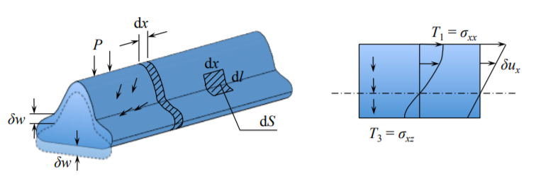
Note that all points on a slice of the beam move downward with the virtual displacement \(\delta w\). The end cuts translate and rotate, according to Equation (1.5.1). Then the right hand side of Equation (2.2.4) becomes

\[\mathrm{RH} = \int_{0}^{l} q\delta w dx + \int_{A} \sigma_{xx} [\delta u^{\circ} - \delta \theta z] dA + \int_{A} \sigma_{xz} \delta w dA \label{2.4.5}\]

where \(q\) is the integrated pressure over the circumference of a slice

\[q = \oint T_iV_i ds \label{2.4.6}\]

and \(V_i\) are direction cosine of the surface traction vector with respect to the \(z\)-axis. In the case of the rectangular section \((h \times b)\), Equation \ref{2.4.6} reduces to

\[q = pb\]

where \(p\) is the distributed pressure on the upper side of the beam and \(q\) is called the line load. The second term in Equation \ref{2.4.5} can be simplified using the definitions Equations (2.2.16-2.2.18)

\[\bar{M} = \int_{A_{\text{end}}} \sigma_{xx} z dA \]

\[\bar{N} = \int_{A_{\text{end}}} \sigma_{xx} dA \]

\[\bar{V} = \int_{A_{\text{end}}} \sigma_{xz} dz\]

where the bar over the symbol indicates that this is the value at the beam end. The final expression for the principle of virtual work for a beam takes the form

\[\int_{0}^{l} \left(N \delta \epsilon^{\circ} + M \delta \kappa\right) d x = \int_{0}^{l} q(x) \delta w d x + \bar{N} \delta u^{\circ} - \bar{M} \delta \theta + \bar{V} \delta w\]

The above principle will be used to derive approximate solutions of the beam problems and also to obtain the equations of equilibrium and boundary conditions.