2.5: Derivation of Equation of Equilibrium for Beams from the Principle of Virtual Work
- Page ID
- 21480

The needed mathematical apparatus is the integration by parts. The starting point in Equation (2.2.6) which is put in an alternative form
\[\frac{da}{dx}b = \frac{d}{dx} (ab) - a\frac{db}{dx}\]
Integrating both sides of the above equation on gets
\[\int \frac{da}{dx}bdx = ab|_{\text{ends}} - \int a\frac{db}{dx} dx\]
To simplify the notation the “prime” convention will be used throughout
\[\frac{d[]}{dx} = {[]}^{\prime}; \; \frac{d^2 []}{dx^2} = {[]}^{\prime\prime}\]
We turn now the left hand side of the principle of virtual work, Equation (2.1.22) and recall the definition of beam curvature and axial strain
\[\kappa = -w^{\prime\prime}\]
\[\epsilon^{\circ} = u^{\prime}\]
The virtual increments are
\[\delta\kappa = -\delta w^{\prime\prime} = (\delta w^{\prime})^{\prime}\]
\[\delta\epsilon^{\circ} = \delta u^{\prime} \label{2.5.7}\]
Substituting Equation \ref{2.5.7} into the LH side of Equation (2.1.22) and integrating twice by parts we get
\[\begin{align} \mathrm{LH} &= - \int_{0}^{l} M (\delta w^{\prime})^{\prime} dx + \int_{0}^{l} N \delta u^{\prime} dx \\[4pt] &= - \left( M \delta w^{\prime} |_{0}^{l} - \int_{0}^{l} M^{\prime} \delta w^{\prime} dx \right) + \left( N \delta u |_{0}^{l} - \int_{0}^{l} N \delta u dx \right) \\[4pt] &= - M \delta w^{\prime} |_{0}^{l} + M^{\prime} \delta w |_{0}^{l} - \int_{0}^{l} M^{\prime\prime} \delta w dx + N\delta u |_{0}^{l} - \int_{0}^{l} N^{\prime} \delta u dx \label{2.5.8} \end{align}\]
The second term represents the work increment at the beam end on downward virtual displacement. Therefore the corresponding generalized force must be the shear force \(V\)
\[V = M^{\prime}\]
Introducing Equation \ref{2.5.8} into Equation (2.4.11) and grouping the terms yields
\[\int_{0}^{l} (M^{\prime\prime} + q)\delta w dx + \int_{0}^{l} N^{\prime} \delta u dx + (M - \bar{M}) \delta w^{\prime} |_{0}^{l} - (N - \bar{N}) \delta u |_{0}^{l} - (V - \bar{V}) \delta w |_{0}^{l} = 0\]
The above equation should hold not for one specific incremental displacement but for arbitrary variations \((\delta w, \delta w^{\prime}, \delta u)\), independent inside \(0 < x < l\) and on the boundaries. Therefore by the first lemma of the calculus of variation, the local (strong) form of the beam equilibrium follows
\[M^{\prime\prime} + q = 0\]
\[N^{\prime} = 0\]
along with the boundary conditions
\[ (M - \bar{M}) \delta w^{\prime} = 0 \]
\[ (V - \bar{V}) \delta u = 0\]
\[ (N - \bar{N}) \delta w = 0\]
In order to satisfy the boundary condition
\[\text{either } M = \bar{M} \text{ or } \delta w^{\prime} = 0 \label{2.5.16}\]
\[\text{either } V = \bar{V} \text{ or } \delta w = 0 \label{2.5.17}\]
\[\text{either } N = \bar{N} \text{ or } \delta u = 0 \label{2.5.18}\]
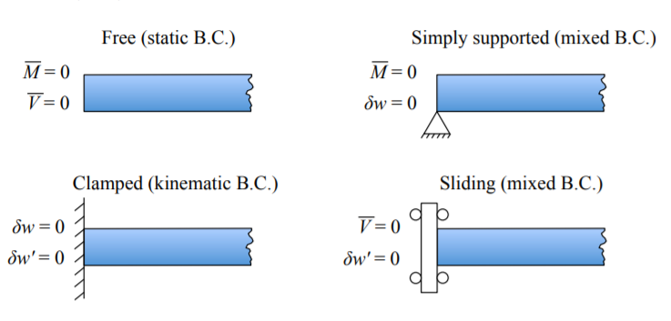
The quantities with a bar denotes the quantities prescribed at the ends of a beam. In particular \(\bar{M}\), \(\bar{V}\), and \(\bar{N}\) could be equal to zero. The first column in Equations \ref{2.5.16}-\ref{2.5.18} represents the static boundary conditions while the second column the kinematic boundary conditions. There are also mixed boundary conditions. The following combinations satisfy all boundary conditions, Figure (\(\PageIndex{1}\)).
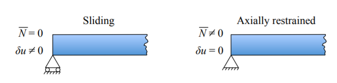
In addition the beam could freely slide at the end along x-axis or can be restrained from sliding, Figure (\(\PageIndex{2}\)).
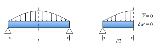
In the case of symmetric loading of the beam, it suffices to consider only one half of the beam with the symmetry boundary condition. The symmetry B.C. is identical to the sliding boundary conditions, as explained in Figure (\(\PageIndex{3}\)).