2.6: Advanced Topic - Mathematical Theory of Beams

The equations of equilibrium of a beam with a rectangular cross-section can be derived in an elegant way from the 3-D equilibrium equation. With zero body forces, the equation of equilibrium in the compact index notation is

\[ \sigma_{ij,j} = 0 \]

or the expanded notation

\[i = 1, \, \sigma_{1j,j} = 0 \rightarrow \sigma_{11,1} + \sigma_{12,2} + \sigma_{13,3} = 0\]

\[i = 2, \, \sigma_{2j,j} = 0 \rightarrow \sigma_{21,1} + \sigma_{22,2} + \sigma_{23,3} = 0\]

\[i = 3, \, \sigma_{3j,j} = 0 \rightarrow \sigma_{31,1} + \sigma_{32,2} + \sigma_{33,3} = 0\]

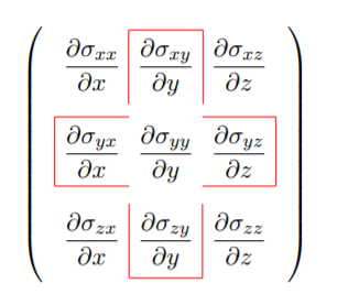
In the engineering notation, the full set of equilibrium equation, already given by Equations (2.1.26-2.1.28), is

\[\label{2.6.5}\]

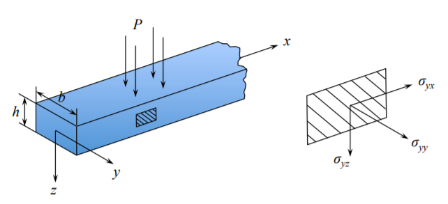
which of the components of the stress tensor will survive beam assumption. Consider a rectangular cross-section beam \((h \times b)\) undergoing planar bending, Figure (\(\PageIndex{1}\)).

The beam is subjected to pressure loading \(p\) at the plane \(z = − \frac{h}{2}\). In the case of planar bending there must be no gradient of stresses in the \(y\)-direction. Therefore the term \(\frac{\partial \sigma_{xy}}{\partial y} = 0\). The surviving components lie outside the shaded box in Equation \ref{2.6.5}, and are:

\[\frac{\partial \sigma_{xx}}{\partial x} + \frac{\partial \sigma_{xz}}{\partial z} = 0 \label{2.6.6}\]

\[\text{Equation in the y-direction is satisfied identically} \label{2.6.7}\]

\[\frac{\partial \sigma_{zx}}{\partial x} + \frac{\partial \sigma_{zz}}{\partial z} = 0 \label{2.6.8}\]

Figure \(\PageIndex{1}\): Vanishing components of the stress vector.

Boundary Conditions

Boundary conditions are specified by the Cauchy formula. The lateral surfaces \(y = \pm \frac{b}{2}\) as well as the lower shelf \(z = \frac{h}{2}\) are stress free. Consider only the upper shelf \(z = −\frac{h}{2}\), defined by the unit normal vector \(\boldsymbol{n}[0, 0, −1]\). Assume that no shear loading is applied, so that the distributed load is directed along \(z\)-axis.

The components of surface traction on the upper shelf are \(\boldsymbol{T}[0, 0, p]\). From the Cauchy formula, calculate the \(z\)-component of the surface traction \( T_3 = \sigma_{3j}n_j = \sigma_{31}n_1 + \sigma_{32}n_2 + \sigma_{33}n_3 \). Only the last term, for which \(n_3 = −1\) remains and so

\[T_3 = p = - \sigma_{33} = -\sigma_{zz}\]

It was straightforward to see that the pressure \(p\) must be equilibrated by the \(\sigma_{zz}\) component. However, for a precise determination of the sign, the Cauchy formula happened to be useful. All other components of the stress tensor on the lateral surface of the beam are zero.

The derivation consists of three steps. First Equation \ref{2.6.6} is integrated with respect to \(z\) and multiplied by the beam width \(b\)

\[\int_{-\frac{h}{2}}^{\frac{h}{2}} \frac{\partial \sigma_{xx}}{\partial x} dz + b \int_{-\frac{h}{2}}^{\frac{h}{2}} \frac{\partial \sigma_{xz}}{\partial z} dz = 0\]

Next, for a definite integral, the differentiation of the integrant in the first is equivalent to the differentiation of the integral. The second term can be integrated to give

\[\int_{-\frac{h}{2}}^{\frac{h}{2}} \sigma_{xx}b dz + \sigma_{xz}|_{-\frac{h}{2}}^{\frac{h}{2}} = 0\]

Noting that \(b dz = dA\), the first integral represents the axial force \(N\), according to the definition, Equation \ref{2.6.7}. The shear stress \(\sigma_{xz}\) is non-zero inside the beam height but vanishes at the lower and upper shelves, \(\sigma_{xz} = 0\), at \(z = \frac{h}{2}\) and \(z = − \frac{h}{2}\). Only the first term survives, which is the force equilibrium in the \(x\)-direction

\[\frac{dN}{dx} = 0 \text{ or } N^{\prime} = 0 \]

In the second step both sides of Equation \ref{2.6.6} are multiplied by \(bz\) and integrated again with respect to \(z\)

\[\int_{-\frac{h}{2}}^{\frac{h}{2}} \frac{\partial \sigma_{xx}}{\partial x} z (b dz) + b \int_{-\frac{h}{2}}^{\frac{h}{2}} \frac{\partial \sigma_{xz}}{\partial z} z (bdz) = 0\]

The second term is now integrated by parts

\[\frac{d}{dx} \int_{-\frac{h}{2}}^{\frac{h}{2}} \sigma_{xx}z dA + \{\sigma_{xz}|_{-\frac{h}{2}}^{\frac{h}{2}} - \int_{-\frac{h}{2}}^{\frac{h}{2}} \sigma_{xz} dA\} = 0\]

The second term vanishes, as before. The first integral is the bending moment \(M\) while the second one-the shear force \(V\) (see the definitions, Equations \ref{2.6.6}-\ref{2.6.8}. So, the above equation represent the moment equilibrium

\[\frac{dM}{dx} − V = 0 \label{2.6.15}\]

In the third, final step, Equation \ref{2.6.15} is integrated with respect to \(z\) after being multiplied by \(b\).

\[\int_{-\frac{h}{2}}^{\frac{h}{2}} \frac{\partial \sigma_{xz}}{\partial x} (b dz) + \int_{-\frac{h}{2}}^{\frac{h}{2}} \frac{\partial \sigma_{zz}}{\partial z} (bdz) = 0\]

After integration one gets

\[\frac{d}{dx} \int_{-\frac{h}{2}}^{\frac{h}{2}} \sigma_{xz} dA + b \left[\sigma_{zz}|_{\frac{h}{2}} - \sigma_{zz}|_{-\frac{h}{2}}\right] = 0 \label{2.6.17}\]

Recalling the boundary condition \(\sigma_{zz}|_{\frac{h}{2}}\) and \(\sigma_{zz}|_{\frac{h}{2}} = −p\), Equation \ref{2.6.17} yields

\[\frac{dV}{dx} + b(−1)(−p) = 0\]

or using \(bp = q\)

\[\frac{dV}{dx} + q = 0 \label{2.6.19}\]

Eliminating the shear force between Equation \ref{2.6.15} and Equation \ref{2.6.19}, the beam equilibrium equation is obtained.

\[\frac{d^2M}{dx^2} + q(x) = 0\]

This equation is identical to the one derived from the principle of virtual work.