
3.2: Elasticity Law in 3-D Continuum
- Page ID
- 21484

The second question is how to extend Equation (3.1.1) to the general 3-D state. Both stress and strain are tensors so one should seek the relation between them as a linear transformation in the form
\[\sigma_{ij} = C_{ij,kl} \epsilon_{kl}\]
where \(C_{ij,kl}\) is the matrix with \(9 \times 9 = 81\) coefficients. Using symmetry properties of the stress and strain tensor and assumption of material isotropy, the number of independent constants are reduced from 81 to just two. These constants, called the Lame’ constants, are denoted by \((\chi, \mu). The general stress strain relation for a linear elastic material is
\[\sigma_{ij} = 2\mu\epsilon_{ij} + \lambda \epsilon_{kk} \delta_{ij} \label{3.2.2}\]
where \(\delta_{ij}\) is the identity matrix, or Kronecker “\(\delta\)”, defined by
\[\delta_{ij} = \begin{vmatrix}
1 & 0 & 0 \\
0 & 1 & 0 \\ 0 & 0 & 1
\end{vmatrix} \text{ or } \begin{array} \delta_{ij} = 1 \; \text{ if } i = j \\ \delta_{ij} = 0 \text{ if } i \neq j \end{array}\]
and \(\epsilon_{kk}\) is, according to the summation convention,
\[\epsilon_{kk} = \epsilon_{11} + \epsilon_{22} + \epsilon_{33} = \frac{dV}{V}\]
In the expanded form, Equation \ref{3.2.2} reads
\[\sigma_{11} = 2\mu \epsilon_{11} + \lambda(\epsilon_{11} + \epsilon_{22} + \epsilon_{33}), \quad \quad \delta_{11} = 1 \label{3.2.5}\]
\[\sigma_{22} = 2\mu \epsilon_{22} + \lambda(\epsilon_{11} + \epsilon_{22} + \epsilon_{33}), \quad \quad \delta_{22} = 1\]
\[\sigma_{33} = 2\mu \epsilon_{33} + \lambda(\epsilon_{11} + \epsilon_{22} + \epsilon_{33}), \quad \quad \delta_{33} = 1\]
\[\sigma_{12} = 2\mu \epsilon_{12} \quad \quad \delta_{12} = 0\]
\[\sigma_{23} = 2\mu \epsilon_{23} \quad \quad \delta_{23} = 0\]
\[\sigma_{31} = 2\mu \epsilon_{31} \quad \quad \delta_{31} = 0 \label{3.2.10}\]
Our task is to express the Lame’ constants by a pair of engineering constants (\(E(\nu)\), where \(\nu\) is the Poisson ratio). For that purpose, we use the virtual experiment of tension of a rectangular bar
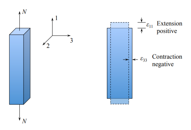
In the conceptual test, measured are the force, displacement and change in the crosssectional dimension. The experimental observations can be summarized as follows:
- \(\sigma_{11}\) is proportional to \(\epsilon_{11}, \sigma_{11} = E\epsilon_{11}\)
- \(\epsilon_{22}\) is proportional to \(\epsilon_{11}, \epsilon_{22} = -\nu\epsilon_{11}\)
- \(\epsilon_{33}\) is proportional to \(\epsilon_{11}, \epsilon_{33} = -\nu\epsilon_{11}\)
Thus the uniaxial tension is producing the one-dimensional state of stress but three-dimensional state of strain
\[ \sigma_{ij} = \begin{vmatrix}
\sigma_{11} & 0 & 0 \\
0 & 0 & 0 \\ 0 & 0 & 0
\end{vmatrix} \; \epsilon_{ij} = \begin{vmatrix}
\epsilon_{11} & 0 & 0 \\
0 & \epsilon_{22} & 0 \\ 0 & 0 & \epsilon_{33}
\end{vmatrix}\]
We introduce now the above information into Equations \ref{3.2.5}-\ref{3.2.10}.
\[\sigma_{11} = 2\mu \epsilon_{11} + \chi(\epsilon_{11} - \nu \epsilon_{11} - \nu\epsilon_{11}) = E\epsilon_{11}\]
\[\sigma_{22} = 2\mu (-\nu\epsilon_{11}) + \chi(\epsilon_{11} - \nu\epsilon_{11} - \nu \epsilon_{11}) = 0\]
and obtain two linear equations relating \((\chi, \mu)\) with \((E, \nu)\)
\[2\mu + \chi(1 − 2\nu) = E \label{3.2.14}\]
\[-2\mu\nu + \chi(1 − 2\nu) = 0 \label{3.2.15}\]
Solving Equations \ref{3.2.14}-\ref{3.2.15} for \(\mu\) and \(\chi\) gives
\[\mu = \frac{E}{2(1 − \nu)}\]
\[\chi = \frac{E\nu}{(1 + \nu)(1 − 2\nu)}\]
The general, 3-D elasticity law, expressed in terms of \((E, \nu)\) is
\[\sigma_{ij} = \frac{E}{1 + \nu} \left[ \epsilon_{ij} + \frac{\nu}{1-2\nu}\epsilon_{kk}\delta_{ij}\right] \label{3.2.18}\]
The mean stress \(p\) where \(−p = \frac{1}{3}\sigma_{kk} = \frac{1}{3} (\sigma_{11} + \sigma_{22} + \sigma_{33})\) is called the hydrostatic pressure. At the same time the sum of the diagonal components of the strain tensor denotes the change of volume. Let us make the so-called “contraction” of the stress tensor in Equation \ref{3.2.18}, meaning that \(i = j = k\)
\[\sigma_{kk} = \frac{E}{1 + \nu} \left[ \epsilon_{kk} + \frac{\nu}{1-2\nu}\epsilon_{kk}\cdot 3\right] \]
where \(\delta_{kk} = (\delta_{11} + \delta_{22} + \delta_{33}) = 1 + 1 + 1 = 3\). From the above equations the following relation is obtained between the hydrostatic pressure and volume change
\[−p = \kappa\frac{dV}{V}\]
where \(\kappa\) is the bulk modulus
\[\kappa = \frac{E}{3(1 − 2\nu)}\]
The elastic material is clearly compressible. It is the crystalline lattice that is compressed but on removal the forces returns to the original volume.
The inverted form of the 3-D Hook’s law is
\[\epsilon_{ij} = \frac{1 + \nu}{E} \sigma_{ij} − \frac{\nu}{E}\sigma_{kk}\delta_{ij}\]
which in terms of the components yields
\[\epsilon_{11} = \frac{1}{E}[\sigma_{11} − \nu(\sigma_{22} + \sigma_{33})] \label{3.2.23}\]
\[\epsilon_{22} = \frac{1}{E}[\sigma_{22} − \nu(\sigma_{11} + \sigma_{33})]\]
\[\epsilon_{33} = \frac{1}{E}[\sigma_{33} − \nu(\sigma_{11} + \sigma_{22})]\]
\[\epsilon_{12} = \frac{1}{2\epsilon}\sigma_{12}\]
\[\epsilon_{23} = \frac{1}{2\epsilon}\sigma_{23}\]
\[\epsilon_{31} = \frac{1}{2\epsilon}\sigma_{31} \label{3.2.28}\]
where \(G = \frac{E}{2(1 + \nu)}\) is called the shear modulus. Equations \ref{3.2.23} - \ref{3.2.28} illustrates the coupling of individual direct strains with all direct (diagonal) components of the stress tensor. At the same time there is no coupling in shear response. The shear strain is proportional to the corresponding shear stress.