7.5: Solution by Taylor expansion
- Page ID
- 21515

Consider the same sample problem of the cantilever beam under the tip point force. Assume the solution as a power series
\[w(x) = \sum^{N}_{n=1} a_n x^n \label{7.5.1}\]
For illustration, truncate the series by taking the four first terms
\[w(x) = a_0 + a_1x + a_2x^2 + a_3x^3 \]
The kinematic boundary conditions are
\[w(x = 0) = 0; \quad w^{\prime}(x = 0) = 0 \]
It is easy to see that displacement boundary conditions are met if \(a_o = a_1 = 0\). The displacements, slopes and curvature become
\[w(x) = a_2x^2 + a_3x^3 \]
\[w^{\prime}(x) = 2a_2x + 3a_3x^2 \]
\[w^{\prime\prime}(x) = 2a_2 + 6a_3x \]
The tip displacement is
\[w(x = l) = w_o = a_2l^2 + a_3l^3 \]
The expression for the total potential energy is
\[\prod = \frac{EI}{2} \int_{0}^{l} (2a + 6a_3x)^2 dx − P(a_2l^2 + a_3l^3 ) \]
or after integration
\[\prod = \frac{EI}{2} (4a^2_2 l + 12a_2a_3l^2 + 12a^2_3 l^3 ) − P(a_2l^2 + a_3l^3 ) \]
The stationary of \(\prod(a_2, a_3)\) implies that
\[\frac{\partial \prod}{\partial a_2} = 0, \quad \frac{\partial \prod}{\partial a_3} = 0 \]
which leads to two linear algebraic equations for \(a_2, a_3\)
\[4a_2 + 6a_3l = \frac{Pl}{EI} \]
\[6a_2 + 12a_3l = \frac{Pl}{EI} \]
where solution is
\[a_2 = \frac{Pl}{2EI}, a_3 = − \frac{P}{6EI} \]
The deflection of the beam is then
\[w(x) = \frac{P}{EI} \left( \frac{lx^2}{2} − \frac{x^3}{6} \right) \]
The tip deflection is obtained
\[w_o = w(x = l) = \frac{Pl^3}{3EI} \]
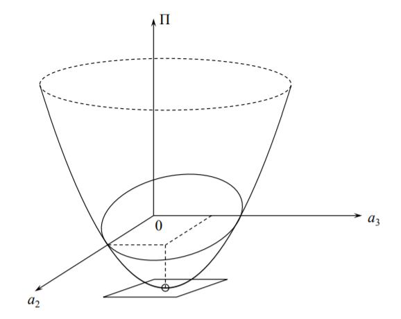
This is the exact solution of the problem. The exact solution was obtained in this case because the first four terms of the Taylor expansion contained the actual deflected shape. Note that the exact solution was obtained by the Ritz method without imposing the static boundary conditions at the tip \(V = −P\) and \(M = 0\). The graphical interpretation of the stationary condition with two degrees of freedom is obtained by plotting Equation \ref{7.5.1} in the space \((\prod, a_2, a_3)\), Figure (\(\PageIndex{1}\)).