7.6: Castigliano Theorem

This theorem applies to statically determined structures and system subjected to concentrated forces or moments. The distribution of bending moments can be uniquely determined from global equilibrium as function of the forces, \(U = U(P)\). The total potential energy is

\[\prod = U(P) − P w_o\]

For a given deflection amplitude \(w_o\), the magnitude of the load adjust itself so as to make the total potential energy stationary. Mathematically

\[\delta [\prod (P)] = \delta [U(P) − P w_o] = \frac{dU}{dP} \delta P − w_o \delta P = \left[ \frac{dU(P)}{dP} − w_o \right] \delta P = 0\]

We have proved that the displacement under the force in the direction of the force is equal to the derivative of the elastic energy stored with respect to the force.

In order to interpret the stationary property of \(\prod\), consider a cantilever beam with the force \(P\) at its tip. The bending moment distribution is \(M(x) = P(l − x)\). Let’s choose the force formulation of the total potential energy, Equation (??). The total potential energy is

\[[\prod = \frac{P^2}{2EI} \int_{0}^{l} (l − x)^2 dx − P w_o \label{8.49}\]

After integration

\[\prod(P) = P \left( \frac{Pl^3}{6EI} − w_o \right) \]

The plot of this function is shown in Fig (\(\PageIndex{1}\)).

Figure \(\PageIndex{1}\): Parabolic variation of the total potential energy with the force \(P\) for a given central deflection.

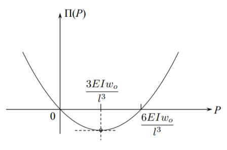
The parabola has two roots at \(P_1 = 0\) and at \(P_2 = \frac{6EIw_o}{l^3}\). The stationary point is at

\[P = \frac{3EIw_o}{l^3} \label{8.51}\]

which is the exact solution of the problem.

As an illustration, consider two simple structural systems. The first system of two beams is shown in Figure (\(\PageIndex{2}\)).

This problem was solved earlier using displacements and slope continuity. A much simple solution follows. The bending moment distributions are

\[\text{ Beam (A) } \; M(x) = −P x \; 0 < x < l \\ \text{ Beam (B) } \; M(x) = \frac{1}{2} P x \; 0 < x < l \\ \text{ Beam (C) } \; M(x) = − \frac{1}{2} P x \; 0 < x < l \]

Figure \(\PageIndex{2}\): Statically determined system and bending moment distribution.

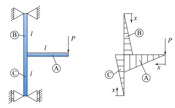
The bending strain energy is

\[U(P) = \int_{0}^{l} \frac{1}{2EI} \left[ P^2 + \left(\frac{P}{2}\right)^2 + \left(\frac{P}{2}\right)^2 \right] x^2 dx = \frac{3}{2} P^2 \frac{l^3}{3} = \frac{1}{2} P^2 l^3 \]

From the relative contributions of the three beams in Equation (7.5.13), it is seen that the horizontal cantilever contributes twice to the tip deflection compared to the vertical beam.

Figure \(\PageIndex{3}\): two welded beams forming an elbow.

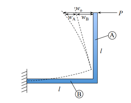
The second system consists of an elbow. From Figure (\(\PageIndex{3}\)), the bending moment distribution is

\[\text{ Beam (A) } \; M(x) = P x \\ \text{ Beam (B) } \; M(x) = Pl \]

The elastic bending energy of the system is

\[U(P) = \frac{1}{2EI} \int_{0}^{l} (P x)^2 dx + \frac{1}{2EI} \int_{0}^{l} (P l)^2 dx = \frac{P^2}{2EI} \frac{4l^3}{3} \]

The total deflection in the direction of the force is

\[w_o = \frac{dU}{dP} = \frac{4}{3} \frac{Pl^3}{EI} \]

Proof of the Castigliano Theorem for a system of point loads, \(P_i\)

The corresponding displacements are denoted by \(w_i\), see Figure (\(\PageIndex{4}\)).

Figure \(\PageIndex{4}\): An elastic body (structure) loaded by a system of concentrated forces.

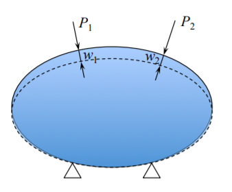
The work of external forces is

\[W = \sum_{i} P_iw_i = P_iw_i \]

It is assumed that the energy stored can be expressed in terms of all the point forces, \(U = U(P_i)\). Let’s keep all point forces at fixed values and vary only one, say \(P_k\). For equilibrium, the total potential energy of the system should be stationary with respect to this change. Thus,

\[\delta \prod = \delta (U - W) = \frac{dU}{dP_k} \delta P_k − w_k \delta P_k \\ = \left( \frac{dU}{dP_k} − w_k \right) \delta P_k = 0\]

The extended Castigliano theorem is

\[w_k = \frac{\partial U(P_i)}{\partial P_k} \]

For example, if there are two point loads applied,

\[w_2 = \frac{\partial U(P_1, P_2)}{\partial P_2} \]

Usually the Castigliano theorem gives only deflection at a given point but not the deflected shape. The extended theorem ca be used to predict the deflected shape.

Figure \(\PageIndex{5}\): Cantilever beam loaded b two point forces.

Illustration

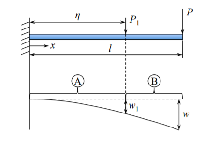
Consider a cantilever beam loaded by two point forces. One force \(P\) is applied at the tip and the other force \(P_1\) acts at a distance \(\eta\) from the support.

The bending moment distribution is

\[\begin{array}{lcl} M_A(x) = P(l − x) + P_1(\eta − x) & \text{ for } & 0 < x < \eta \\ M_B(x) = P(l − x) & \text{ for } & \eta< x < l \end{array}\]

The bending strain energy is

\[U(P, P_1) = \frac{1}{2EI} \int_{0}^{\eta} M^2_{A} dx + \frac{1}{2EI} \int_{\eta}^{l} M^2_B dx \]

According to Equation \ref{8.49}, the deflection under the point load \(P_1\) is

\[w_1 = \frac{\partial U(P, P_1)}{\partial P_1} = \frac{1}{EI} \int_{0}^{\eta} M_A \frac{\partial M_A}{\partial P_1} dx + \frac{1}{EI} \int_{\eta}^{l} M_B \frac{\partial M_B}{\partial P_1} dx\]

The derivatives of the bending moments are

\[\frac{\partial M_A}{\partial P_1} = \eta − x \]

\[\frac{\partial M_B}{\partial P_1} = 0 \]

Substituting Equations \ref{8.51} and (??) into (??), one gets

\[w_1 = \frac{1}{EI} \int_{0}^{\eta} [P(l − x) + P_1(\eta − x)](\eta − x) dx \]

This equation is valid for any combination of \(P\) and \(P_1\). We can therefore assume that \(P_1\) is a “dummy” force and can be set equal to zero. Then, Equation (??) reduces to

\[w_1 = \frac{1}{EI} \int_{0}^{\eta} [P(l − x)(\eta − x) dx \]

which gives, after integration,

\[w_1(\eta) = \frac{Pl^3}{3EI} \left[ \frac{3}{2} \left(\frac{\eta}{l}\right)^2 − \frac{1}{2} \left(\frac{\eta}{l}\right)^3 \right] \]

In the above solution \(\eta\) is an arbitrary position along the beam and \(w_1(\eta)\) is the corresponding deflection. By changing the variables

\[\eta \rightarrow x \\ w_1(\eta) = w(x) \]

we can recover the exact deflected shape of the cantilever beam

\[w_1(\eta) = \frac{Pl^3}{3EI} \left[ \frac{3}{2} \left(\frac{x}{l}\right)^2 − \frac{1}{2} \left(\frac{x}{l}\right)^3 \right] \]

The above example illustrated a great flexibility of the Castigliano method in solving statically determined problems.