9.4: Dynamic Snap-Through

The present lecture notes are restricted to static and quasi-static problems. However, the nature of the snap-through problem calls for the consideration of the full dynamic analysis. Assume that the loading of the two-bar system is load controlled. There is a stable equilibrium path on the portion AB. When \(\bar{P}_{\text{max}} = \frac{2}{3 \sqrt{3}}\bar{\delta}^3\) is reached, the system jumps instantaneously to the next equilibrium point F in the static solution. The magnitude of the force is the same, but the corresponding displacement is determined from the solution of the cubic equation

\[\frac{2}{3\sqrt{3}}\bar{\delta}^3 = \delta \bar{\delta}^2 − \delta^3 \]

This equation has three real roots

\[\delta_1 = \frac{\bar{\delta}}{\sqrt{3}}, \delta_2 = \delta_3 = − \frac{2 \bar{\delta}}{\sqrt{3}} \]

By adding inertia forces into the equation of equilibrium, the snap-through process occurs in time. The bar system is first accelerated on the portion BCD of the descending force and then decelerated on the rising portion DEF.

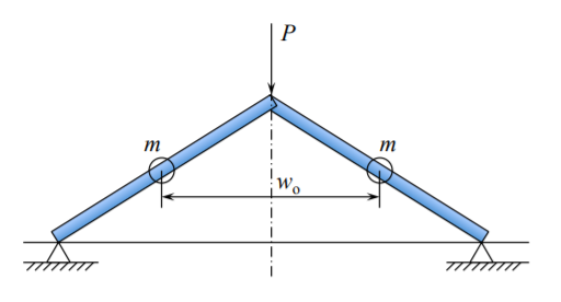
The dynamic solution is straight forward if the distributed mass of the rod is lumped into two discrete point masses \(m = lA\rho\), as shown in Figure (\(\PageIndex{1}\)).

By adding d’Alambert inertia forces into static equilibrium, Equation (9.3.5), one gets

\[−P − 2m \frac{\ddot{w}_o}{2} = 2N \frac{w_o}{l} \label{10.52}\]

where now \(P\) is positive in tension.

Figure \(\PageIndex{1}\): The equivalent two massless bars and two lumped masses.

Eliminating the axial force \(N\) in the bars between Equations (9.3.4) and \ref{10.52}, one gets the following differential equation

\[−\bar{P} − \frac{l^2 \rho}{E} \ddot{\delta} = \delta [ \delta^2 − \bar{\delta}^2 ] \label{10.53}\]

where the dot denotes differentiation with respect to time. It is convenient to introduce the dimensionless time \(\bar{t} = \frac{t}{t_1}\), where \(t_1 = \frac{l}{c}\) is the reference time, and \(c^2 = \frac{E}{\rho}\) is the speed of the longitudinal stress wave in a bar. In the force controlled system, the exciting term is constant \(\bar{P} = \frac{2}{3 \sqrt{3}}\bar{\delta}^3\). In the new dimensionless coordinate, Equation \ref{10.53} takes the form

\[−\bar{P} − \ddot{\delta} = \delta^3 − \bar{\delta}^2 \delta \label{10.54}\]

where the dot denotes differentiation with respect to the dimensionless time \(\bar{t}\). Using the chain rule of differentiation,

\[\ddot{\delta} = \frac{d \dot{\delta}}{d\bar{t}} = \frac{d \dot{\delta}}{d\delta} \frac{d \delta}{d\bar{t}} = \frac{d \dot{\delta}}{d\delta} \dot{\delta} \label{10.55}\]

one can get a solution on the phase plane \((\delta, \dot{\delta}\)) rather tan in the time domain. Substituting Equation \ref{10.55} into Equation \ref{10.54}, the following equation is obtained

\[−\bar{P} d\delta − \dot{\delta}d \dot{\delta} = (\delta^3 − \bar{\delta}^2 \delta ) d\delta \]

which can be readily integrated to give

\[−\bar{P} \delta − \frac{1}{2} \dot{\delta}^2 = \frac{\delta^4}{4} − \frac{\bar{\delta^2}\delta^2}{2} + C \label{10.57}\]

The integration constant \(C\) is determined from the initial condition that the velocity \(\dot{\delta}\) is zero when the deflection reaches \(\delta = \frac{1}{\sqrt{3}}\) (point B). The solution for the velocity \(\dot{\delta}\) is

\[\dot{\delta} = 2\bar{\delta}^2 \sqrt{−P \left(\frac{\delta}{\bar{\delta}}\right) + \frac{1}{2}\left(\frac{\delta}{\bar{\delta}}\right)^2 − \frac{1}{4} \left(\frac{\delta}{\bar{\delta}}\right)^4 + \frac{1}{12}} \label{10.58}\]

In terms of the normalized velocity \(\frac{\dot{\delta}}{2 \bar{\delta}^2} = \bar{v}\) and the normalized deflection \(\eta = \frac{\delta}{\bar{\delta}}\), Equation \ref{10.58} reads

\[\bar{v} = \sqrt{−\frac{2}{3 \sqrt{3}}\eta + \frac{1}{2}\eta^2 − \frac{1}{4}\eta^4 + \frac{1}{12}} \label{10.59}\]

The plot of \(\bar{v}\) versus \(\eta\) is shown in Figure (\(\PageIndex{2}\)).

Figure \(\PageIndex{2}\): The plot of \(\bar{v}\) versus \(\eta\) in dynamic snap through.

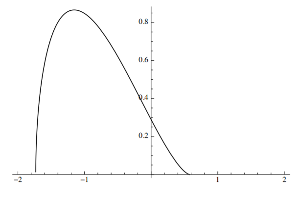
The polynomial in \(\eta\) under the square root in Equation \ref{10.59} has two real roots, at \(\eta = \frac{1}{\sqrt{3}}\) and \(\eta = − \sqrt{3}\). The dynamic motion starts at B, increases slowly, reaches a maximum in F and falls rapidly to zero at the point G with the coordinate \(\eta_f = \sqrt{3}\). Note that the dynamic deflection overshoots considerably the deflection reached in the static problem \(\eta_{\text{stat}} = \frac{2}{\sqrt{3}} = 1.15\).

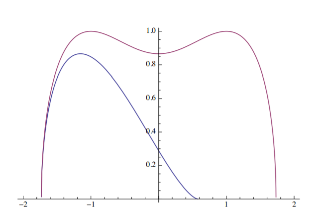
At the final stage when the motion of the system stops, there is enough tensile energy stored in the bar to initial free vibration with the forcing term \(\bar{P}\) removed. The solution to this phase is given by Equation \ref{10.57} with \(\bar{P} = 0\), and the new integration constant \(C_1 = \frac{3}{4}\) so that continuity of velocity is achieved. The plot of the free vibration of the system, governed by

\[\bar{v} = \sqrt{\frac{1}{2}\eta^2 − \frac{1}{4}\eta^4 + \frac{3}{4}} \]

is shown in Figure (\(\PageIndex{3}\)), in comparison with the dynamic snap-through plot.

Figure \(\PageIndex{3}\): The plot of \(\bar{v}\) versus \(\eta\) in free vibration, in comparison with the dynamic-through plot.