
10.1: Governing Equations and Boundary Conditions
- Page ID
- 21532

In the present notes the column buckling was extensively studied in Chapter 8. The governing equation for a geometrically perfect column is
\[EIw^{\mathrm{IV}} + Nw^{\prime\prime} = 0 \]
A step-by-step derivation of the plate buckling equation was presented in Chapter 6
\[D\nabla^4w + \bar{N}_{\alpha\beta}w_{,\alpha\beta} = 0 \]
where \(N_{\alpha\beta}\) is a set of constant, known parameters that must satisfy the governing equation of the pre-buckling state, given by Equations (6.1.10-6.1.12). The classical buckling analysis of plates is best explained on an example of a rectangular plate subjected to compressive loading in one direction, Figure (\(\PageIndex{1}\)).
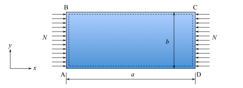
The plate is simply supported along all four edges. The edges AB and CD are called the loaded edges because in-plane loading \(N\left[\frac{N}{M}\right]\) is applied to these edges. The other two edges AD and BC are called the unloaded edges. The simply supported boundary conditions apply to vanishing of transverse deflections and the normal bending moments
\[w = 0 \quad \text{ on ABCD} \label{10.1.3}\]
\[M_n = 0 \quad \text{ on ABCD} \label{10.1.4}\]
Separate boundary condition must be formulated in the in-plane direction in the normal and tangential direction
\[(N_n − \bar{N}_n)\delta u_n = 0 \]
\[(N_t − \bar{N}_t)\delta u_t = 0 \]
In the case of the present rectangular plate Equations \ref{10.1.3} - \ref{10.1.4} reduce to
\[\left.\begin{array}{l} \left(N_{x x}-\bar{N}_{x x}\right) \delta u_{x}=0 \\ \left(N_{x y}-\bar{N}_{x y}\right) \delta u_{y}=0 \end{array}\right\} \text { on AB and CD } \\ \left.\begin{array}{l} \left(N_{y y}-\bar{N}_{y y}\right) \delta u_{y}=0 \\ \left(N_{x y}-\bar{N}_{x y}\right) \delta u_{x}=0 \end{array}\right\} \text { on AD and BC } \]
In the present problem the stress boundary conditions are applied and the tensor of external loading is
\[\bar{N}_{\alpha\beta} = \begin{vmatrix} \bar{N} & 0 \\ 0 & 0 \end{vmatrix}, \quad N_{\alpha\beta} = \begin{vmatrix} N & 0 \\ 0 & 0 \end{vmatrix} \]
With the above field of membrane forces the equilibrium equations are satisfied identically. From the constitutive equations
\[N_{xx} = C(\epsilon_{xx}^{\circ} + \nu\epsilon_{yy}^{\circ}) \]
\[0 = C(\epsilon_{yy}^{\circ} + \nu\epsilon_{xx}^{\circ}) \]
Therefore \(\epsilon_{yy}^{\circ} = −\nu\epsilon_{xx}^{\circ}\) and so \(N_{xx} = Eh\epsilon_{xx}^{\circ}\). The displacement is calculated by solving two equations
\[\epsilon_{xx}^{\circ} = \frac{du_x}{dx} \]
\[\epsilon_{yy}^{\circ} = \frac{du_y}{dy} \]
With the origin of the coordinate system placed at the point A in Figure (\(\PageIndex{1}\)), The solution is
\[u_x = u_o \left( 1 − \frac{x}{a} \right), \quad u_y = \nu u_o \frac{y}{a}, \quad N = \frac{Eh}{a} u_o \]
Note that \(\bar{N}\) has been defined as positive in compression. Therefore the plate will be compressed in the x-direction and will expand laterally in the y-direction because of the effect of the Poison ratio. In setting up the experiment or developing the FE model, the plate should be left free in the in-plane direction.