Engineering LibreTexts

10.4: Buckling of Sections

  • Page ID
    21535
  • \( \newcommand{\vecs}[1]{\overset { \scriptstyle \rightharpoonup} {\mathbf{#1}} } \)

    \( \newcommand{\vecd}[1]{\overset{-\!-\!\rightharpoonup}{\vphantom{a}\smash {#1}}} \)

    \( \newcommand{\dsum}{\displaystyle\sum\limits} \)

    \( \newcommand{\dint}{\displaystyle\int\limits} \)

    \( \newcommand{\dlim}{\displaystyle\lim\limits} \)

    \( \newcommand{\id}{\mathrm{id}}\) \( \newcommand{\Span}{\mathrm{span}}\)

    ( \newcommand{\kernel}{\mathrm{null}\,}\) \( \newcommand{\range}{\mathrm{range}\,}\)

    \( \newcommand{\RealPart}{\mathrm{Re}}\) \( \newcommand{\ImaginaryPart}{\mathrm{Im}}\)

    \( \newcommand{\Argument}{\mathrm{Arg}}\) \( \newcommand{\norm}[1]{\| #1 \|}\)

    \( \newcommand{\inner}[2]{\langle #1, #2 \rangle}\)

    \( \newcommand{\Span}{\mathrm{span}}\)

    \( \newcommand{\id}{\mathrm{id}}\)

    \( \newcommand{\Span}{\mathrm{span}}\)

    \( \newcommand{\kernel}{\mathrm{null}\,}\)

    \( \newcommand{\range}{\mathrm{range}\,}\)

    \( \newcommand{\RealPart}{\mathrm{Re}}\)

    \( \newcommand{\ImaginaryPart}{\mathrm{Im}}\)

    \( \newcommand{\Argument}{\mathrm{Arg}}\)

    \( \newcommand{\norm}[1]{\| #1 \|}\)

    \( \newcommand{\inner}[2]{\langle #1, #2 \rangle}\)

    \( \newcommand{\Span}{\mathrm{span}}\) \( \newcommand{\AA}{\unicode[.8,0]{x212B}}\)

    \( \newcommand{\vectorA}[1]{\vec{#1}}      % arrow\)

    \( \newcommand{\vectorAt}[1]{\vec{\text{#1}}}      % arrow\)

    \( \newcommand{\vectorB}[1]{\overset { \scriptstyle \rightharpoonup} {\mathbf{#1}} } \)

    \( \newcommand{\vectorC}[1]{\textbf{#1}} \)

    \( \newcommand{\vectorD}[1]{\overrightarrow{#1}} \)

    \( \newcommand{\vectorDt}[1]{\overrightarrow{\text{#1}}} \)

    \( \newcommand{\vectE}[1]{\overset{-\!-\!\rightharpoonup}{\vphantom{a}\smash{\mathbf {#1}}}} \)

    \( \newcommand{\vecs}[1]{\overset { \scriptstyle \rightharpoonup} {\mathbf{#1}} } \)

    \(\newcommand{\longvect}{\overrightarrow}\)

    \( \newcommand{\vecd}[1]{\overset{-\!-\!\rightharpoonup}{\vphantom{a}\smash {#1}}} \)

    \(\newcommand{\avec}{\mathbf a}\) \(\newcommand{\bvec}{\mathbf b}\) \(\newcommand{\cvec}{\mathbf c}\) \(\newcommand{\dvec}{\mathbf d}\) \(\newcommand{\dtil}{\widetilde{\mathbf d}}\) \(\newcommand{\evec}{\mathbf e}\) \(\newcommand{\fvec}{\mathbf f}\) \(\newcommand{\nvec}{\mathbf n}\) \(\newcommand{\pvec}{\mathbf p}\) \(\newcommand{\qvec}{\mathbf q}\) \(\newcommand{\svec}{\mathbf s}\) \(\newcommand{\tvec}{\mathbf t}\) \(\newcommand{\uvec}{\mathbf u}\) \(\newcommand{\vvec}{\mathbf v}\) \(\newcommand{\wvec}{\mathbf w}\) \(\newcommand{\xvec}{\mathbf x}\) \(\newcommand{\yvec}{\mathbf y}\) \(\newcommand{\zvec}{\mathbf z}\) \(\newcommand{\rvec}{\mathbf r}\) \(\newcommand{\mvec}{\mathbf m}\) \(\newcommand{\zerovec}{\mathbf 0}\) \(\newcommand{\onevec}{\mathbf 1}\) \(\newcommand{\real}{\mathbb R}\) \(\newcommand{\twovec}[2]{\left[\begin{array}{r}#1 \\ #2 \end{array}\right]}\) \(\newcommand{\ctwovec}[2]{\left[\begin{array}{c}#1 \\ #2 \end{array}\right]}\) \(\newcommand{\threevec}[3]{\left[\begin{array}{r}#1 \\ #2 \\ #3 \end{array}\right]}\) \(\newcommand{\cthreevec}[3]{\left[\begin{array}{c}#1 \\ #2 \\ #3 \end{array}\right]}\) \(\newcommand{\fourvec}[4]{\left[\begin{array}{r}#1 \\ #2 \\ #3 \\ #4 \end{array}\right]}\) \(\newcommand{\cfourvec}[4]{\left[\begin{array}{c}#1 \\ #2 \\ #3 \\ #4 \end{array}\right]}\) \(\newcommand{\fivevec}[5]{\left[\begin{array}{r}#1 \\ #2 \\ #3 \\ #4 \\ #5 \\ \end{array}\right]}\) \(\newcommand{\cfivevec}[5]{\left[\begin{array}{c}#1 \\ #2 \\ #3 \\ #4 \\ #5 \\ \end{array}\right]}\) \(\newcommand{\mattwo}[4]{\left[\begin{array}{rr}#1 \amp #2 \\ #3 \amp #4 \\ \end{array}\right]}\) \(\newcommand{\laspan}[1]{\text{Span}\{#1\}}\) \(\newcommand{\bcal}{\cal B}\) \(\newcommand{\ccal}{\cal C}\) \(\newcommand{\scal}{\cal S}\) \(\newcommand{\wcal}{\cal W}\) \(\newcommand{\ecal}{\cal E}\) \(\newcommand{\coords}[2]{\left\{#1\right\}_{#2}}\) \(\newcommand{\gray}[1]{\color{gray}{#1}}\) \(\newcommand{\lgray}[1]{\color{lightgray}{#1}}\) \(\newcommand{\rank}{\operatorname{rank}}\) \(\newcommand{\row}{\text{Row}}\) \(\newcommand{\col}{\text{Col}}\) \(\renewcommand{\row}{\text{Row}}\) \(\newcommand{\nul}{\text{Nul}}\) \(\newcommand{\var}{\text{Var}}\) \(\newcommand{\corr}{\text{corr}}\) \(\newcommand{\len}[1]{\left|#1\right|}\) \(\newcommand{\bbar}{\overline{\bvec}}\) \(\newcommand{\bhat}{\widehat{\bvec}}\) \(\newcommand{\bperp}{\bvec^\perp}\) \(\newcommand{\xhat}{\widehat{\xvec}}\) \(\newcommand{\vhat}{\widehat{\vvec}}\) \(\newcommand{\uhat}{\widehat{\uvec}}\) \(\newcommand{\what}{\widehat{\wvec}}\) \(\newcommand{\Sighat}{\widehat{\Sigma}}\) \(\newcommand{\lt}{<}\) \(\newcommand{\gt}{>}\) \(\newcommand{\amp}{&}\) \(\definecolor{fillinmathshade}{gray}{0.9}\)

    Cold-form or welded profiles are encountered in almost every aspect of the engineering practice. Typical cross-sectional geometries of prismatic members are shown in Figure (\(\PageIndex{6}\)).

    Graph showing curves of critical stiffness (kc) against aspect ratio (a/b) for various support conditions labeled A to E.
    Figure \(\PageIndex{1}\): Effect of boundary conditions on the buckling coefficient of rectangular plates subjected to in-plane boundary conditions.
    Diagram of a 3D angle structure on the left with labels A, B, and C, and a 2D angle representation on the right.
    Figure \(\PageIndex{2}\): Buckling mode of an angle element.
    3D rectangular prism on the left labeled with dimensions 'a' and 'b'; right shows a dashed outline of the prism's base.
    Figure \(\PageIndex{3}\): The buckling mode of a prismatic square column.
    Diagram showing a 3D structure with a curved surface on the left and an angled flat surface on the right, labeled with dimensions.
    Figure \(\PageIndex{4}\): Buckling due to shear or bending.
    Wavy metal sheet with grid pattern and holes, showing signs of wear and rust.
    Figure \(\PageIndex{5}\): A photograph of shear buckling of a plate representing the damage pattern on the ship’s hull inflicted upon grounding.
    Text art spelling "LUTRIC" with various geometric shapes and lines in a minimalist style.
    Figure \(\PageIndex{6}\): Some typical open and closed cross-sectional shape of prismatic members.

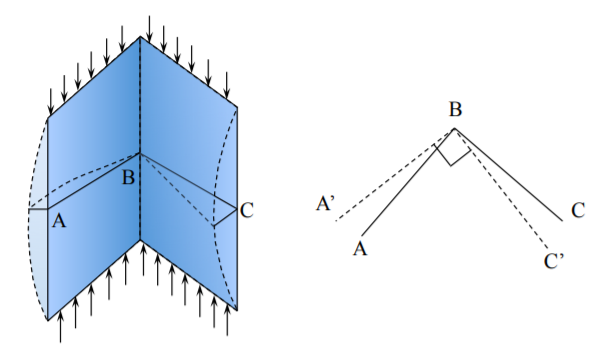
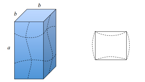
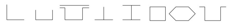
    Except of symmetric angle, “T”, cruciform and square box profile where buckling strength of the entire section is a sum of buckling loads of contributing plates, the analysis of other shape requires consideration of restraining bending moments and continuity conditions along the common edges. The easiest way to illustrate the problem is to consider a rectangular section prismatic column, Figure (\(\PageIndex{7}\)). According to Equation (??) the buckling load is inversely proportional to the width of the plate. The two opposite wider plates would like to buckle first, but the shorter sides are not ready to buckle with \(k = 4\). They provide clamped boundary condition for the wider flanges for which \(k \cong 7\). There must be a transfer of information between the adjacent plates so that they will buckle “in sympathy” to one another with a different \(k_c\).

    Graph showing the relationship between k and the ratio b2/b1, with labeled curves k1, k2 and points b1, b2.
    Figure \(\PageIndex{7}\): Buckling coefficients of a rectangular plate as a function of \(b_2/b_1\).

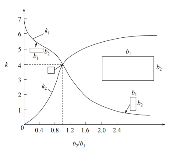
    The numerically obtained function \(k_1(b_2/b_1)\) is shown in Figure (\(\PageIndex{7}\)) by a solid line. The buckling coefficient is uniquely related to \(k_1\) through the pre-buckling analysis. Before buckling the strains and compressive stresses in the adjacent plates are the same

    \[\sigma_1 = \frac{N_1}{h_1} = \sigma_2 \frac{N_2}{h_2}\]

    where

    \[N_1 = k_1 \frac{\pi^2 D_1}{b^2_1}, \quad N_2 = k_2 \frac{\pi^2 D_2}{b^2_2}\]

    From the above equation it follows that

    \[k_2 = k_1 \left( \frac{b_2}{b_1} \right)^2\]

    \(k_1\) is shown in Figure (\(\PageIndex{7}\)) (solid line). The buckling coefficient \(k_2\) calculated from Equation (??) is shown on the same figure by the dashed line. With the above result one can prove that for a given weight (cross-section area) the square column will have the largest buckling resistance for all rectangular shapes.

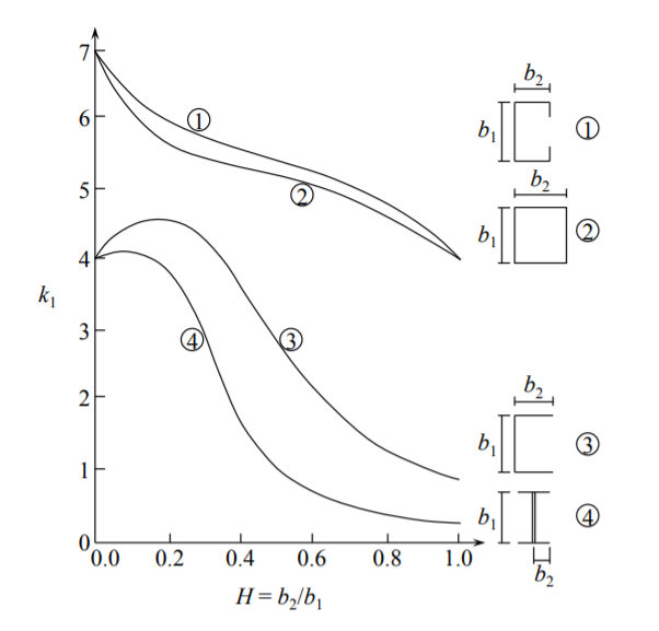
    For more complex cross-sectional shape the buckling coefficient can be presented in a graphical form, as shown in Figure (\(\PageIndex{8}\)). Knowing the buckling coefficient \(k_1\) for a flange with the width \(b_1\) and thickness \(h_1\), the buckling coefficients of all other flanges is then calculated from:

    \[k_i = k_1 \left(\frac{h_ib_1}{h_1b_i}\right)\]

    In most cases nothing dramatic happens at the point of buckling. The purely compressive state switches into a combined bending/compression but the plate continues to carry additional load with a reduced stiffness. The post-buckling and ultimate load response is discussed in the next section of this chapter.

    Graph showing k1 vs. H (b2/b1) with four labeled curves and corresponding diagrams of b1 and b2 configurations.
    Figure \(\PageIndex{8}\): Buckling coefficients for four types of sections.

    This page titled 10.4: Buckling of Sections is shared under a CC BY-NC-SA 4.0 license and was authored, remixed, and/or curated by Tomasz Wierzbicki (MIT OpenCourseWare) via source content that was edited to the style and standards of the LibreTexts platform.