10.6: Ultimate Strength of Plates

In the previous section we have shown that after buckling the plate continues to take additional load but with half of its pre-buckling stiffness. In order to understand what happens next, let’s examine the distribution of in-plane compressive stresses \(\sigma_{xx}\) at \(x = a\). From Equations (10.2.10-10.2.11) and (??) the components \(\sigma_{xx}\) is

\[\sigma_{xx}(y) = \frac{N_{xx}}{h} = \frac{E}{1 − \nu^2} \left[ −(1 − \nu^2) \frac{u_o}{a} + \frac{\pi^2}{2} \left(\frac{w_o}{a} \right)^2 \sin^2 \frac{\pi y}{a} \right] \]

The first term represents negative, compressive stress, uniform along the width of the plate. The second term describes the relieving tensile stress produced by finite rotation. The relation between \(w_o\) and \(u_o\) is given by Equation (??) and is depicted in Figure (10.5.2). A plot of the function \(\sigma_{xx}(y)\) for several values of the time-like parameter \(u_o\) is shown in Figure (\(\PageIndex{1}\)). Note that the curves labeled A, B, C and D corresponds to the respective points in Figs. (10.5.2) and (10.5.3).

Figure \(\PageIndex{1}\): Re-distribution of compressive stresses along the loaded edge and simple approximation by von Karman.

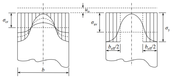
With increasing plate compression there is a re-distribution of stresses along the loaded edge \(x = 0\) and \(x = a\). The stress at the unloaded edge \(y = 0\) and \(y = a\) keeps increasing while the stress at the plate symmetry plane \(y = \frac{a}{2}\) diminishes to zero.

It was the German scientist and engineer, Theodore von Karman who in 1932 made use of the observation presented in Figure (\(\PageIndex{1}\)). He assumed that the central, unloaded portion of the plate carries zero stress while the edge zone, each of the width \(b_{\text{eff}}/2\) reaches the yield stress at the point of ultimate load. As a starting point, von Karman used the expression for the critical buckling load \(N_c\) and looked at the relation between the stress at the loaded edge \(\sigma_e\) and the plate width \(b\)

\[\sigma_e = \frac{N_e}{h} = \frac{N_c}{h} = \frac{4\pi^2D}{hb^2} = \frac{4\pi^2Eh^2}{12(1 − \nu^2)b^2} = 1.9^2E\left(\frac{h}{b}\right)^2\]

Normally \(b\) is the input parameter and the stress \(\sigma_e\) is an unknown quantity. The ingenuity of von Karman was that he inverted what is known and unknown in Equation (??). He asked what should be the width of the plate \(b_{\text{eff}}\) so that the edge stress reaches the yield stress. Thus

\[\sigma_y = 1.9^2E\left(\frac{h}{b_{\text{eff}}}\right)^2\]

Solving the above equation for \(b_{\text{eff}}\)

\[b_{\text{eff}} = 1.9h \sqrt{\frac{E}{\sigma_y}}\]

Taking for example \(E = 200000\) MPa, \(b_{\text{eff}}\sigma_y = 320\) MPa, the effective width becomes

\[b_{\text{eff}} = 1.9h \sqrt{625} = 47.5h \]

The effective width depends on the Young’s modulus and yield stress is proportional to the plate thickness. Approximately 40-50 thicknesses of the plate near the edges carries the load, the remaining central part is not effective. The total load on the plate can be expressed in two ways

\[P_{\text{ult}} = b_{\text{eff}} \cdot \sigma_y = b \cdot \sigma_{\text{av}}\]

where \(\sigma_{\text{av}} = \sigma_{\text{ult}}\) is the average stress on the loaded edge at the point of ultimate strength,

\[\frac{\sigma_{\text{av}}}{\sigma_{\text{ult}}} = \frac{b_{\text{eff}}}{b} = 1.9 \frac{h}{b} \sqrt{\frac{E}{\sigma_y}}\]

The group of parameters

\[\beta = \frac{b}{h} \sqrt{\frac{\sigma_y}{E}}\]

is referred to as the slenderness ratio of the plate. Note that this is a different concept than the slenderness ratio of the column \(l/\rho\). Using the parameter \(\beta\), the ultimate strength of the plate normalized by the yield stress is

\[\frac{\sigma_{\text{ult}}}{\sigma_{y}} = \frac{1.9}{\beta}\]

Recall that the normalized buckling stress of the elastic plate is

\[\frac{\sigma_{\text{cr}}}{\sigma_{y}} = \left(\frac{1.9}{\beta}\right)^2\]

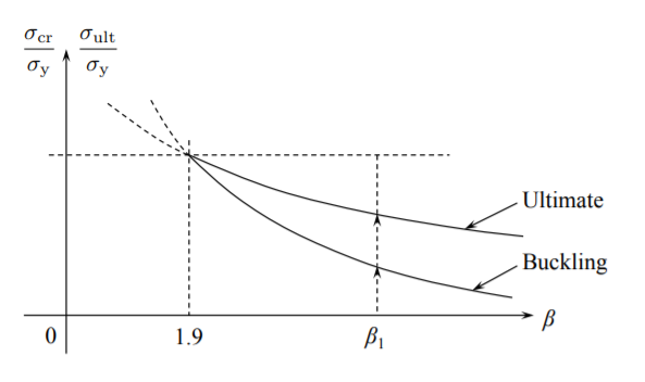
Plots of both functions are shown in Figure (\(\PageIndex{2}\)).

From this figure one can identify the critical slenderness ratio

\[\beta_{\text{cr}} = 1.9 \]

when both the ultimate load and the critical buckling load reach yield. From Equation (??) one can see that at \(\beta = \beta_{\text{cr}}\), the effective width is equal to the plate width, \(b_{\text{eff}} = b\).

Figure \(\PageIndex{2}\): Dependence of the buckling stress and ultimate stress on the slenderness ratio.

Eliminating the parameter \(\beta\) between Equations (??) and (??), the ultimate stress is seen to be the geometrical average between the yield stress and critical buckling stress

\[\sigma_{\text{ult}} = \sqrt{\sigma_{\text{cr}} \cdot \sigma_{y}}\]

For example, continuous loading of a plate with the slenderness ratio \(\beta_1\) will first encounter the buckling curve and then the ultimate strength curve, as illustrated in Figure (\(\PageIndex{2}\)). The foregoing analysis was valid for plates simply supported along all four edges, for which the buckling coefficient is \(k_c = 4\). For other type of support Equation (??) is still valid with the coefficient 1.9 replaced by 1.9 \(\frac{k_c}{4}\).

Much effort has been devoted in the past to validate experimentally the prediction of the von Karman effective width theory. It was found that a small correction to Equation (??) provides good fit of most of the test data

\[\frac{\sigma_{\text{ult}}}{\sigma_{y}} = \frac{b_{\text{eff}}}{b} = \frac{1.9}{\beta} − \frac{0.9}{\beta^2}\]

For example, for a relatively short (stocky plate) \(\beta = 2\beta_{\text{cr}} = 3.8\), the original formula over predicts by 15% than the more exact empirical equation (??). For slender plates, the difference is small. The latter has been the basis for the design of thin-walled compressive elements in most domestic and international standards such as AISI, Aluminum Association and AISC.