11.1: Hardening Curve and Yield Curve

If we go to the lab and perform a standard tensile test on a round specimen or a flat dogbone specimen made of steel or aluminum, most probably the engineering stress-strain curve will look like the one shown in Figure (\(\PageIndex{1a}\)). The following features can be distinguished:

Point A - proportionality limit

Point B - 0.02% yield

Point C - arbitrary point on the hardening curve showing different trajectories on loading/unloading

Point D - fully unloaded specimen

For most of material the initial portion of the stress-strain curve is straight up to the proportionality limit, point A. From this stage on the stress-strain curve becomes slightly curved but there is no distinct yield point with a sudden change of slope. There is in international standard the yield stress is mapped by taking elastic slope with 0.02% strain \((\epsilon = 0.0002)\) offset strain.

Figure \(\PageIndex{1}\): Elastic, plastic and total stress-strain curve.

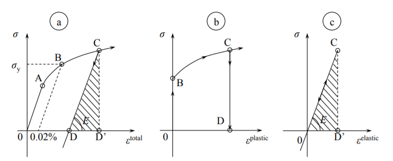
Upon loading, the material hardens and the stress is increasing with diminishing slop until the testing machine (either force or displacement controlled) is stopped. There are two possibilities. On unloading, meaning reversing the load or displacement of the cross-load of the testing machine, the unloading trajectory is straight. This is the elastic unloading where the slop of the stress-strain curve is equal to the initial slope, given by the Young’s modulus. At point D the stress is zero but there is a residual plastic strain of the magnitude OD. The experiment on loading/unloading tell us that the total strain \(\epsilon^{\text{total}}\) can be considered as the sum of the plastic strain \(\epsilon^{\text{plastic}}\) and elastic strain \(\epsilon^{\text{elastic}}\). Thus

\[\epsilon^{\text{total}} = \epsilon^{\text{plastic}} + \epsilon^{\text{elastic}}\]

The elastic component is not constant but depends on the current stress

\[\epsilon^{\text{elastic}} = \frac{\sigma}{E} \]

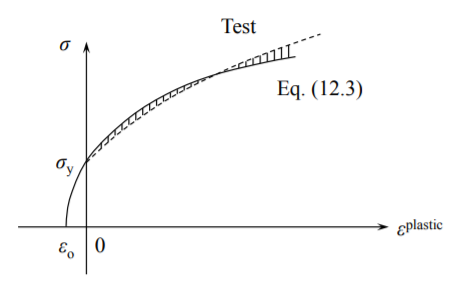
The plastic strain depends on how far a given specimen is loaded, and thus there is a difference between the total (measured) strain and known elastic strain. Various empirical formulas were suggested in the literature to fit the measured relation between the stress and the plastic strain. The most common is the swift hardening law

\[\sigma = A(\epsilon^{\text{plastic}} + \epsilon_o)^n\]

where \(A\) is the stress amplitude, \(n\) is the hardening exponent and \(\epsilon_o\) is the strain shift parameter.

In many practical problems the magnitude of plastic strain is mud larger than the parameter \(\epsilon_o\), giving rise to a simpler power hardening law, extensively used in the literature.

\[\sigma = A \epsilon^n \]

For most metals the exponent \(n\) is the range of \(n = 0.1 - 0.3\), and the amplitude can vary a lot, depending on the grade of steel. A description of the reverse loading and cycling plastic loading is beyond the scope of the present lecture notes.

Figure \(\PageIndex{2}\): The experimentally measured stress-strain curve and the fit by the swift law.

Various other approximation of the actual stress-strain curve of the material are in common use and some of then are shown in Figure (\(\PageIndex{3}\)).

Figure \(\PageIndex{3}\): Elastic-linear hardening material (a) and rigid-plastic hardening material (b).

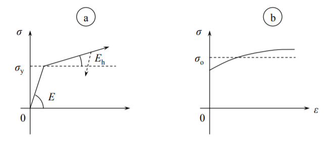
A further simplification is obtained by considering the average value \(\sigma_o\) of the stress-strain curve, illustrated in Figure (\(\PageIndex{3b}\)). This concept gave rise to the concept of the rigid-perfectly plastic material characteristic time, depicted in Figure (11.2.1).

The material model shown in Figure (11.2.1) is adopted in the development of the limit analysis of structures. The extension of the concept of the hardening curve to the 3-D case will be presented later, after deriving the expression for the yield condition.