7.2: Graphical Representations of Metal Solubility
- Page ID
- 39550
This page is a draft and is under active development.
Metal-Hydroxide Precipitation
Solubility and precipitation reactions typically involve a metal cation in solution bonding with a corresponding counter anion, which could be monatomic (Cl-, F-) or polyatomic (CO3-2, PO4-3). One anion commonly involved in precipitation is the hydroxide ion, OH-. We also know that hydroxide is a key player in acid-base equilibria and the pH scale. So, it comes to reason that the solubility of metals is influenced by the pH state of an aqueous system.
A metal cation of charge +n will generally react with n hydroxide ions to form a neutral precipitate of the form \[\ce{Me(OH)_{n(s)}}\] which can be represented with the following equation:
\[\ce{ Me_{n(s)} \rightleftharpoons Me^{+n}_{(aq)} + nOH^{-}_{(aq)}} \nonumber\]
If we use the equation for Ksp in combination with the equation for Kw, we can reveal the relationship between metal hydroxide solubility and pH. Let’s use an example of magnesium hydroxide, \[\ce{Mg(OH)_{2}}\] ...for which Ksp = 5.61x10^-12 (engineeringtoolbox.com). Starting with the solubility equilibrium expression for Ksp:
\[ K_{sp}=[\ce{Mg^{+2}_{(aq)}}][\ce{OH^{-}_{(aq)}}]^2 \nonumber\]
If we take the log_10 of both sides of the equation and rearrange:
\[ log(K_{sp})=log[\ce{Mg^{+2}}]+2 log[\ce{OH^{-}}] \nonumber\]
\[ log[\ce{Mg^{+2}}]=log(K_{sp})-2 log[\ce{OH^{-}}] \nonumber\]
\[ log[\ce{Mg^{+2}}]=log(K_{sp}) + 2 pOH \nonumber\]
We know that pH + pOH = 14, so pOH = 14-pH. Also, the log_10 of Ksp = -11.25. Substituting those into the equation below yields
\[ log[\ce{Mg^{+2}}]= -11.25 + 2 (14 – pH) \nonumber\]
\[ log[\ce{Mg^{+2}}]= -11.25 + 28 – 2pH \nonumber\]
\[ log[\ce{Mg^{+2}}]= 16.75 – 2pH \nonumber\]
Or, if we multiply by -1, the left hand side is -log[Mg+2], or pC for Mg+2.
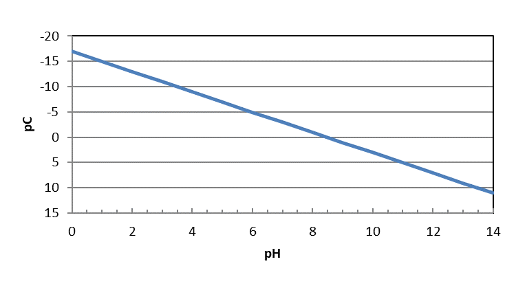
\[ -log[\ce{Mg^{+2}}]= -16.75 + 2pH \nonumber\]
This equation shows the relationship between the maximum concentration of dissolved magnesium in aqueous solution as a function of pH. The concentration is a maximum because it was derived from the Ksp equation, which represents the limit of solubility. It should be noted that this equation does not consider the presence of other anions that might precipitate with magnesium, only hydroxide ion.
We can show this relationship graphically by plotting the concentration against pH as the independent variable. With acids and bases, we plotted pC-pH diagrams, or the -log of the concentration on the y-axis. Then, we flipped the y-axis so that it preserved the concept of high concentrations being high on the y-axis and low concentrations low on that axis.
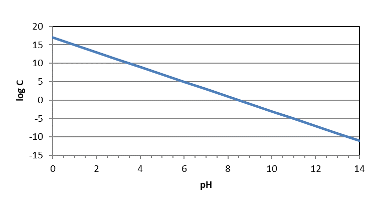
You may also see these figures plotted as logC-pH diagrams. However, they should look exactly the same except for the numeric quantities on the y-axis. In logC-pH diagrams, the y-axis will appear as it would on a normal figure – with higher numbers at the top and lower at the bottom. Because those are logC values instead of pC (-logC) values, concentrations are still higher at the top of the diagram and lower at the bottom of the diagram.
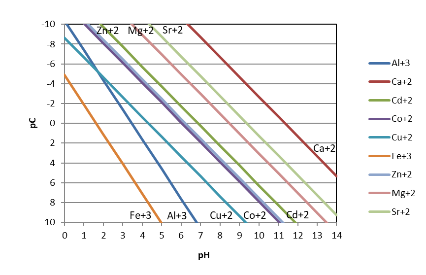
If we follow this approach for multiple metal ions, we can compare the relative solubilities of metal hydroxides as a function of pH. Examining the figure below, we see two general observations. First, metal hydroxides can be present at much higher concentrations at lower pH. In other words, metal hydroxides are more soluble under acidic conditions. This makes sense when we consider Le Chatelier’s principle: at low pH values, hydroxide ion (one of the products of the dissolution reaction) is very scarce in solution. So, the dissolution equilibrium should ‘want’ to shift to the right towards the products of hydroxide and the dissolve metal ion. A second observation from the figure is that, at a given pH, trivalent metal ions (aluminum and ferric iron) are less soluble than divalent metal ions.