6.2.2: Inductance and Inductors

To begin, we need to examine the interrelation between electric current and magnetic fields in a conductor. When a current passes through a conductor, such as a wire, a magnetic field is created around the conductor that is proportional to the strength of the current. This is illustrated in Figure 9.2.1 .

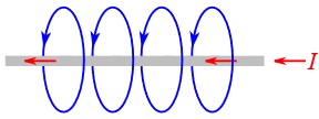
Figure 9.2.1 : Magnetic field around a conductor.

The magnetic field can be thought of as sets of concentric rings around the conductor, although for clarity only single loops are drawn in the Figure. The number of magnetic lines in a given area is known as the magnetic flux and is given the symbol \(\Phi\) (the Greek letter phi). The unit of magnetic flux is the weber, Wb, named after Wilhelm Weber, a 19th century German physicist.

\[\text{Magnetic flux } \equiv \text{ the number of magnetic lines enclosed in a given area.} \label{9.1} \]

Note that the magnetic field runs the length of the conductor. The direction of the field lines follows the right hand rule: if you grasp the wire with your right hand such that your thumb is pointing in the direction of conventional current flow, then your fingers wrap in the direction of the magnetic field. This rule is illustrated in Figure 9.2.2 .

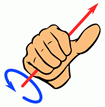
Figure 9.2.2 : Right hand rule. Image source (modified)

If we form the conductor into a loop, the field lines are corralled into the center of the loop. This is illustrated in Figure 9.2.3 . In this diagram it can be seen that the lines effectively collect in the center, going into the page.

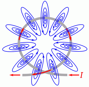
Figure 9.2.3 : Magnetic field around a loop.

The enhancement effect can be magnified by adding more loops in tandem. This is known as a solenoid and is shown in Figure 9.2.4 . It is the most basic form of an inductor.

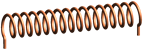
Figure 9.2.4 : Solenoid.

The concentrating effect of the magnetic field is shown in Figure 9.2.5 . In this figure, the coil is shown from the side, as a cross-section of the individual loops. The dots inside the conductors indicate that the current is flowing toward you, out of the page; while the the crosses indicate that the current is flowing into the page. The lines of flux exit out the right, loop around, and reenter from the left. Due to limited space, the entire loop for each line is not drawn, and it is important to remember that magnetic flux lines do not end, but always create a loop. Further, although it is shown as a plane here, this field is three dimensional, with lines looping back into the page as well as in front of it.

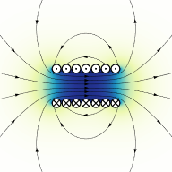
Figure 9.2.5 : Magnetic field in a solenoid. Image source

This is how electromagnets can be created¹. The north pole is the exiting end (right side) of Figure 9.2.5 while the south pole is the entering end (left side).

If the current changes, there will be a commensurate change in the magnetic field. Further, this change in the field will induce a current in the conductor that creates a magnetic field that opposes the original change in the field. This is known as Lenz's law. Alternately, it can be stated that the induced current caused by a changing magnetic field will oppose the change in the original current that created that change in the original magnetic field.

At this point we can offer a proper definition of the weber:

\[1 \text{ weber } \equiv \text{ the magnetic flux that, acting on a single loop of a conductor, produces a potential of 1 volt if the flux is reduced to zero at an even rate over 1 second.} \label{9.2} \]

In magnetic circuits we are also interested in the magnetic flux density which is the magnetic flux per unit area. The symbol for flux density is \(B\) and has units of teslas (T), named after Nicola Tesla, the Serbo-Croatian-American engineer and inventor. One tesla is defined as one weber per square meter.

\[1 \text{ tesla } \equiv 1 \text{ weber} / \text{meter}^2 \label{9.3} \]

To provide a reference, the magnetic flux density of the Earth near the equator is approximately 31 \(\mu\)T, while the value of the voice coil gap in a loudspeaker is around 1 to 2 T, with medical MRI scanners being a little higher still.

Finally, we come to the definition of inductance and its unit, the henry:

\[\text{Inductance is a measure of the tendency of a conductor to oppose a change in the current flowing through it.} \label{9.4} \]

\[1 \text{ henry } \equiv 1 \text{ weber} / 1 \text{ amp} \label{9.5} \]

Unsurprisingly, the energy stored in the magnetic field of an inductor is proportional to the inductance. It is also proportional to the square of the current through the inductor.

\[W = \frac{1}{2} L I^2 \label{9.6} \]

Where

\(W\) is the energy in joules,

\(L\) is the inductance in henries,

\(I\) is the current in amps.

Figure 9.2.6 : Simple air-core inductor dimensions.

An inductor in its simplest form consists of a series of wire loops. These might be wound around an iron core, although a non-ferrous core might also be used. For a simple single layer inductor, such as the one drawn in Figure 9.2.6 , the inductance is described by the following formula:

\[L=\mu \frac{A N^2}{l} \label{9.7} \]

Where

\(L\) is the inductance in henries,

\(\mu\) is the permeability of the core material,

\(A\) is the cross sectional area of the coil,

\(N\) is the number of coils or turns,

\(l\) is the length of the coil.

Inductors may also be wound using multiple layers or around a toroidal core, and these designs utilize alternate formulas.

Inductor Styles and Packaging

Equation \ref{9.7} indicates that, in order to achieve high inductance, we would like a core with high permeability, permeability being a measure of how easy it is to establish magnetic flux in said material. Substances such as iron or ferrite have a much greater permeability than air and are used commonly for cores. They do have a disadvantage in that they will saturate sooner than an air core, and this can lead to distortion.

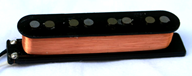
Figure 9.2.7 : Electric bass guitar pickup.

Another approach is to pack as many turns as is possible within a given length. One way to do this is to minimize the thickness of the insulation around the wire². This can be achieved by using a thin enamel coating instead of the typical plastic insulation. A second method is to use a very fine wire. This leads to two problems, namely an undesirable increase in equivalent series resistance (known colloquially as coil resistance or \(R_{coil}\)), and limited current carrying capacity. All of these effects have to be balanced in order to achieve the best performance for a given application.

Commercial inductors range in value from a fraction of a nanohenry for small surface mount “chip” inductors up to several henries. Some devices exhibit large internal inductances even though they are not specifically used as inductors. One common example is a transformer. Another example is an electric guitar or bass pickup, such as the one shown in Figure 9.2.7 with its cover removed. Units such as this may be constructed of several thousand turns of very fine wire (typically AWG 41 to 44) and achieve inductances in excess of one henry.

A variety of inductors is shown in Figure 9.2.9 , all of which are of the through-hole type (surface mount inductors do not appear considerably different from their surface mount resistor and capacitor cousins).

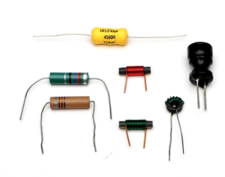
Figure 9.2.9 : A collection of inductors.

The two units toward the left are molded inductors and use a standard color code, similar to the ones used for resistors and capacitors. The unit at the top (yellow) is a high current inductor that features low \(R_{coil}\). The three inductors in the center use obvious ferrite cores, two wound on straight cores and the third wound on a toroidal core. The unit to the right uses a high permeability material at the very top and is wrapped in a plastic sheath for protection. Variable inductors are also a possibility and can be made by using a ferrite core that can be slid within the coils, effectively changing the permeability of the core (part ferrite, part air).

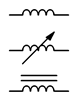
Figure 9.2.10 : Inductor schematic symbols (top-bottom): standard, variable, iron/ferrite core.

The schematic symbols for inductors are shown in Figure 9.2.10 . The standard symbol is at the top. The variable inductor symbol is in the middle and is a twolead device, somewhat reminiscent of the symbol for a rheostat. At the bottom is the symbol for an inductor with an iron, ferrite, or similar high permeability core. In general, like resistors, single inductors are not polarized and cannot be inserted into a circuit backwards. There are, however, special applications where multiple coils can be wound on a common core, and for these, the polarity of their interconnection can make a difference.

Inductor Data Sheet

A portion of an inductor data sheet is shown in Figure 9.2.12 . This page lists the available sizes of this particular model, each with corresponding quantities. We can see this model is available in inductance values ranging from 1 \(\mu\)H up to 100 mH. Tolerance of the smaller values is \(\pm\)10% while values at and above 33 \(\mu\)H are at \(\pm\)5%. \(Q\) is the quality factor and is particularly important in AC circuits (higher being better), along with its associated frequency, \(f_Q\). Continuing across we find \(I_R\). This is the maximum rated current. For the smaller values, we find they can withstand in excess of 2 amps while the larger units can withstand only tens of milliamps.

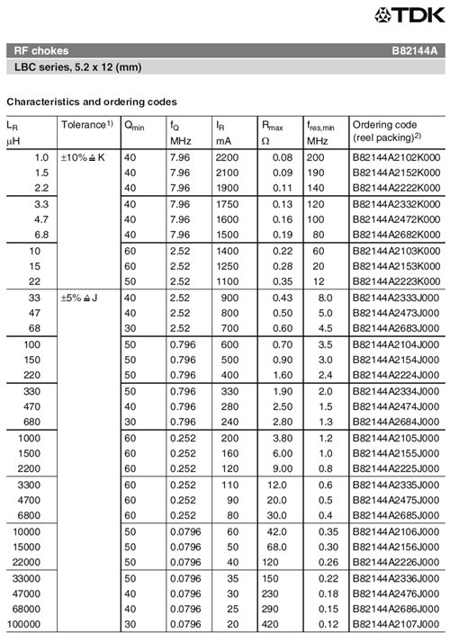
Figure 9.2.12 : Inductor data sheet. Courtesy of TDK

Finally, we come to \(R_{max}\). This is also known as \(R_{coil}\). It represents the equivalent series resistance of the inductor. In general, smaller is better. For this model, it ranges from a fraction of an ohm to a few hundred ohms. This trend is typical of inductors; all else being equal, the larger the inductance, the larger the value of the associated series resistance. In many circuits, the value of \(R_{coil}\) cannot be ignored.

Inductors in Series and in Parallel

Suppose we take two identical inductors and place them in series. This effectively doubles both the length and the number of loops. From Equation \ref{9.7} we can see that doubling both the number of loops and the length would double the inductance. This is because \(N^2\) goes up by a factor of four which is then halved be the increased length. Consequently, inductors in series add values just like resistors in series. By extension, inductors in parallel behave like resistors in parallel. The equivalent of parallel inductors can be found by using either the product-sum rule or by taking the reciprocal of the sum of their reciprocals.

Example 9.2.1

Find the equivalent inductance of the network shown in Figure 9.2.11 .

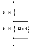
Figure 9.2.11 : Circuit for Example 9.2.1 .

The 6 mH and 12 mH inductors are in parallel. The equivalent value of the pair is:

\[L_{parallel} = \frac{L_2 L_3}{L_2+L_3} \nonumber \]

\[L_{parallel} = \frac{6 mH12 mH}{6 mH+12 mH} \nonumber \]

\[L_{parallel} = 4mH \nonumber \]

This combination is in series with the 5 mH inductor. Therefore the total equivalent inductance is 4 mH + 5 mH, or 9 mH.

Current-Voltage Relationship

The fundamental current-voltage relationship of the inductor is the mirror image of that of the capacitor:

\[\mathcal{v} = L \frac{di}{dt} \label{9.8} \]

This states that the voltage across the inductor is a function of how quickly the current is changing. If the current is not changing (i.e., in steady-state), then the voltage across the inductor is zero. In this case, the inductor behaves like a short, or more accurately, like its \(R_{coil}\) value. In contrast, during a rapid initial current change, the inductor voltage can be large, and thus the inductor behaves like an open.

If we rearrange Equation \ref{9.8} and solve for the rate of change of current, we find that:

\[\frac{di}{dt} = \frac{\mathcal{v}}{L} \label{9.9} \]

Thus if an inductor is fed by a constant voltage source, the current will rise at a constant rate equal to \(\mathcal{v}/L\). For example, considering the circuit in Figure 9.2.11 , we see a voltage source feeding a single inductor. If we were to plot the inductor's current over time, we would see something like the graph of Figure 9.2.12 .

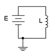
Figure 9.2.11 : Inductor with voltage source.

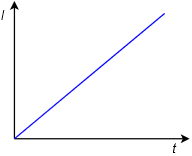
Figure 9.2.12 : Inductor current versus time.

As time progresses, the current through the inductor increases, flowing from top to bottom. With a theoretically perfect inductor and source, this would continue as long as the circuit was energized. In reality, this line would either begin to deflect horizontally as the source reached its limits, or the inductor would fail once its maximum current or power handling was reached. The slope of this line is dictated by the size of the applied voltage source and the inductance.

Example 9.2.2

Determine the rate of change of current through the inductor in the circuit of Figure 9.2.13 . Also determine the inductor's current 10 microseconds after power is switched on.

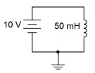
Figure 9.2.13 : Circuit for Example 9.2.2 .

From Equation \ref{9.9}, the rate of change of current is:

\[\frac{di}{dt} = \frac{\mathcal{v}}{L} \nonumber \]

\[\frac{di}{dt} = \frac{10V}{50 mH} \nonumber \]

\[\frac{di}{dt} = 200 A \text{ per second} \nonumber \]

In other words, for every second, the current rises another 200 amps. Thus, after just 10 microseconds it will have risen to 200 A/s times 10 \(\mu\)s, or 2 mA.

Equation \ref{9.8} is key to understanding the behavior of inductors. As noted previously, if an inductor is driven by a fixed voltage source and ignoring \(R_{coil}\), the current through it rises at the constant rate of \(\mathcal{v}/L\). This change in current through the inductor is not limitless. An instantaneous change requires that \(di/dt\) is infinite, and thus, the voltage driving the inductor would also have to be infinite, which is a clear impossibility. Therefore we can state a particularly important characteristic of capacitors:

\[\text{The current through an inductor cannot change instantaneously.} \label{9.10} \]

This observation will be central to analyzing the operation of inductors in DC circuits.

References

¹Truly one of the coolest inventions of all time: a magnet with an on/off switch.

²The wound wire must be insulated otherwise each loop will short to the loops next to it and we'd be left with a tube instead of a series of loops.