4.6: Maximum Power Transfer Theorem

Given a simple voltage source with internal resistance, a useful question to ask is “What value of load resistance will yield the maximum amount of power in the load?” While it is not true that maximizing load power is a goal of all circuit designs, it is a goal of a portion of them and thus worth a closer look. Consider the basic circuit depicted in Figure 6.6.1 with source \(E\), source internal resistance \(R_i\) and load resistance \(R\).

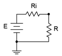
Figure 6.6.1 : Defining maximum power transfer.

We would like to describe the load power in terms of the load resistance. To make the job easier, we may normalize the voltage source \(E\) to 1 volt and the source resistance \(R_i\) to 1 Ohm. By doing this, \(R\) also becomes a normalized value, that is, it no longer represents a simple resistance value but rather represents a ratio in comparison to \(R_i\). In this way the analysis will work for any set of source values. Note that the value of \(E\) will equally scale the power in both \(R_i\) and \(R\), so a precise value is not needed, and thus, we may as well chose 1 volt for convenience.

The power in the load can be determined by using \(I^2 R\) where \(I = E / (R_i+R)\). Using our normalized values \(I = 1 / (1+R)\) and thus the load power is:

\[P = \left( \frac{1}{1+R} \right)^2 R \text{ or after expanding, } P = \frac{R}{R^2+2 R+1} \nonumber \]

We now have an equation that describes the load power in terms of the load resistance. Before we go any further, take a look at what this equation tells you, in general. It is obvious that maximum power will not occur at the extremes. If \(R = 0\) or \(R = \infty \) (i.e., shorted or opened load) the load power is zero. While shorting the load will yield the maximum load current, it will also yield zero load voltage and thus no power. Similarly, opening the load will yield maximum load voltage but it will also yield zero load current, and again, no load power. To find the precise value that produces the maximum load power, the proof can be divided into two major portions. The first involves graphing the function and the second requires differential calculus to solve for a precise value. We shall proceed with the graphing portion which will lead us to the answer. The more rigorous proof of the second method is detailed in Appendix C.

Graphing the Power Function \(P = R / (R^2+2R+1)\)

This may be done in parts, looking at the contribution of each term, and then combining to form the final result. First, consider the denominator \(R^2 + 2R + 1\). It consists of three segments. The most simple is the horizontal line at +1. The \(2R\) term creates a straight line with slope 2 starting at the origin. The \(R^2\) term creates a simple curve with increasing slope that starts at the origin, crosses the horizontal +1 line at \(R = 1\) and also crosses the \(2R\) line at \(R = 2\). These items are drawn individually and then added together as illustrated in Figure 6.6.2 .

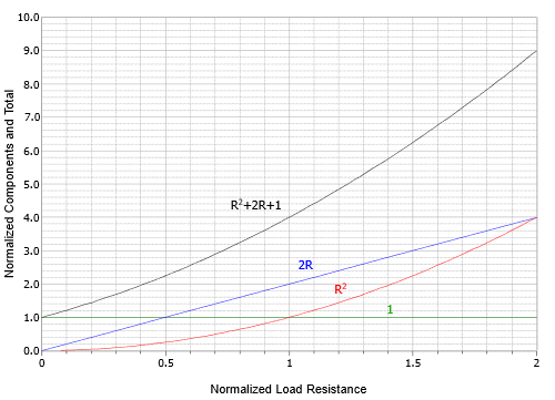
Figure 6.6.2 : The three terms of the power equation plotted individually and then summed.

Of course, we must remember that we really want \(1 / ( R^2 + 2R + 1)\) and so we plot the reciprocal of the combo as shown in Figure 6.6.3 (red curve). We also include the numerator term, \(R\). This is shown as a straight line (blue) with a slope of 1. Finally, these two curves are multiplied together to produce the load power equation (black).

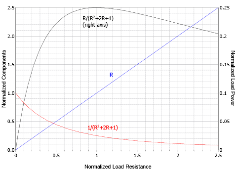
Figure 6.6.3 : The power equation and components plotted.

A close examination of the power curve will show that the peak occurs at \(R = 1\). This is easier to see if we plot the completed power curve using a logarithmic horizontal axis and also scale the vertical axis to 100%, as shown in Figure 6.6.4 . The peak is more apparent and the curve is symmetrical in shape rather than lopsided. This reinforces the idea that the ratio of the resistances is what matters.

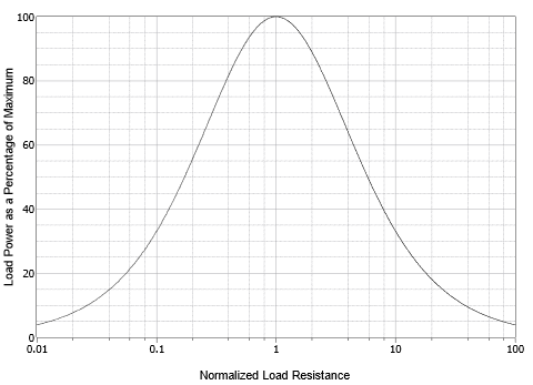
Figure 6.6.4 : The load power curve with logarithmic axis showing symmetry.

Finally, we can state:

\[\text{Maximum load power will be achieved when the load resistance is equal to the internal resistance of the driving source.} \nonumber \]

No other value of load resistance will produce a higher load power. For the circuit of Figure 6.6.1 , this means that \(R\) must equal \(R_i\). As an exercise, we can try substituting a few values around the peak to verify this. For example, given \(E\) = 1 V and \(R_i\) = 1 \(\Omega\), we calculate \(P\) for \(R\) = 0.5 \(\Omega\), 1 \(\Omega\), and 2 \(\Omega\):

\[P_{0.5} = 0.5/(0.5^2+2 \cdot 0.5+1) = 2/9 \nonumber \]

\[P_1 = 1/(1^2+2 \cdot 1+1) = 2/8 = 1/4 \nonumber \]

\[P_2 = 2/(2^2+2 \cdot 2+1) = 2/9 \nonumber \]

You can also try this with extremely small variations such as \(R\) = 0.9999 \(\Omega\) along with \(R\) = 1.0001 \(\Omega\) and you will not achieve a value equal to or greater than 1/4 Watt.

While matching the resistance produces the maximum load power, it does not produce maximum load current or maximum load voltage. In fact, this condition produces a load voltage and a load current that are half of their maximums. Their product, however, is at the maximum. Further, efficiency at maximum load power is only 50% (i.e., only half of all generated power goes to the load with the other half being wasted internally). Values of \(R\) greater than \(R_i\) will achieve higher efficiency but at reduced load power. Sometimes we favor efficiency over maximal load power.

As any linear two point network can be reduced to something like Figure 6.6.1 by using Thévenin's theorem, combining the two theorems allows us to determine maximum power conditions for any resistor in a complex circuit.