
4.7: Advanced Topic- Delta-Y Conversions
- Page ID
- 52913

Certain component configurations, such as bridged networks, cannot be reduced to a single resistance using basic series-parallel conversion techniques. One method for simplification involves converting sections into more convenient forms. The configurations in question are three-point networks containing three resistors. Due to the manner in which they drawn, they are referred to as delta networks and Y networks1. These configurations are shown in Figures 6.7.1 . In this particular case the delta version is drawn upside down so that its terminal designations match those of the Y configuration.
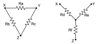
Figure 6.7.1 : Delta and Y (\(\Delta\)-Y) networks.
Alternately, if they are slightly redrawn they are known as pi (also called “\(\pi\)”) networks and T (also called “tee”) networks. These configurations are shown in Figure 6.7.2 .
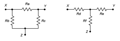
Figure 6.7.2 : Alternate form: Pi and T(\(\pi\)-T) networks.
It is possible to convert back and forth between delta and Y networks. That is, for every delta network, there exists a Y network such that the resistances seen between the X, Y and Z terminals are identical, and vice versa. Consequently, one configuration can replace another in order to simplify a larger circuit.
\(\Delta\)-Y Conversion
A true equivalent circuit would present the same resistance between any two terminals as the original circuit. Consider the unloaded case for the circuits of Figure 6.7.1 (i.e., just these networks with nothing else connected to them). The equivalent resistances seen between each pair of terminals for the delta and Y respectively are:
\[R_{XY} = R_a || (R_b+R_c) = R_d + R_e \label{6.1} \]
\[R_{XZ} = R_b || (R_a+R_c) = R_d + R_f \label{6.2} \]
\[R_{ZY} = R_c || (R_b+R_a) = R_e + R_f \label{6.3} \]
Assuming we have the delta and are looking for the Y equivalent, note that we have three equations with three unknowns (\(R_d\), \(R_e\) and \(R_f\)). Thus, they can be solved using a term elimination process. If we subtract Equation \ref{6.3} from Equation \ref{6.1} we eliminate the second resistance (\(R_e\)) and arrive at a difference between the first and third unknown resistances (\(R_d − R_f\)). This quantity can then be added to Equation \ref{6.2} to eliminate the third resistance (\(R_f\)), leaving just the first unknown resistance (\(R_d\)).
\[(R_d + R_e) − (R_e + R_f) = (R_d − R_f) = R_a || (R_b+R_c) − R_b || (R_a+R_c) \nonumber \]
\[(R_d + R_f) + (R_d − R_f) = 2R_d = 2( R_b || (R_a+R_c) + R_a || (R_b+R_c) − R_c || (R_a+R_b) ) \nonumber \]
Therefore,
\[R_d = R_b || (R_a+R_c) + R_a || (R_b+R_c) − R_c || (R_a+R_b) \nonumber \]
which, after simplifying, is:
\[R_d = \frac{R_a R_b}{R_a+R_b+R_c} \label{6.4} \]
Similarly, we can show that
\[R_e = \frac{R_a R_c}{R_a+R_b+R_c} \label{6.5} \]
\[R_f = \frac{R_b R_c}{R_a+R_b+R_c} \label{6.6} \]
Note that if three identical resistors are used, the values of the Y equivalent will all be one-third of that value.
Helpful Hint for Remembering \(\Delta\)-Y Conversion Equations
Examine the equations for \(R_d\), \(R_e\), and \(R_f\). You will note that they all have the same denominator. What kind of mnemonic (memory helper) can you come up with to help you remember the relationship between the resistor whose value you are trying to calculate and the resistors in the numerator on the right-hand side of the equation.
Suggestion
- The resistances in the numerator are the two resistors in the delta network that are connected to the same node as the resistor in the Wye network whose value you are trying to determine.
- For example, if you are calculating \(R_d\), you'll notice it is connected to node \(X\). In the delta configuration, \(R_a\) and \(R_b\) are connected to node \(X\), so the product of \(R_a\) and \(R_b\) is used in the calculation of \(R_d\)
Y-\(\Delta\) Conversion
For the reverse process of converting Y to delta, start by noting the similarities of the expressions for \(R_d\), \(R_e\) and \(R_f\). If two of these expressions are divided, a single equation for \(R_a\), \(R_b\) or \(R_c\) will result. For example, using Equations \ref{6.4} and \ref{6.5}:
\[\frac{R_d}{R_e} = \frac{\frac{R_a R_b}{R_a+R_b+R_c}}{\frac{R_a R_c}{R_a+R_b+R_c}} \nonumber \]
\[\frac{R_d}{R_e} = \frac{R_a R_b}{R_a R_c} \nonumber \]
\[\frac{R_d}{R_e} = \frac{R_b}{R_c} \nonumber \]
Therefore,
\[\frac{R_b}{R_c} = \frac{R_d}{R_e} \nonumber \]
\[R_b = \frac{R_c R_d}{R_e} \nonumber \]
This process can be repeated for Equations \ref{6.4} and \ref{6.6} to obtain an expression for \(R_a\). The two expressions for \(R_a\) and \(R_b\) can then be substituted into Equation \ref{6.4} to obtain an expression for \(R_c\) that utilizes only \(R_d\), \(R_e\) and \(R_f\). A similar process is followed for \(R_a\) and \(R_b\) resulting in:
\[R_a = \frac{R_d R_e+R_e R_f +R_d R_f}{R_f} \label{6.7} \]
\[R_b = \frac{R_d R_e+R_e R_f +R_d R_f}{R_e} \label{6.8} \]
\[R_c = \frac{R_d R_e+R_e R_f +R_d R_f}{R_d} \label{6.9} \]
If three identical resistors are used, the values of the delta equivalent will all be three times that value, the inverse of the situation when converting from delta to Y.
Helpful Hint for Remembering Y-\(\Delta\) Conversion Equations
Examine the equations for \(R_a\), \(R_b\), and \(R_c\). You will note that they all have the same numerator.
What kind of mnemonic can you come up with to help you remember the relationship between the resistor whose value you are trying to calculate and the resistor in the denominator on the right-hand side of the equation.
Suggestion
- The resistance in the denominator is the value of the resistor in the Wye network that is connected to the node opposite the resistor in the Delta network whose value you are trying to determine
- For example, if you are calculating \(R_a\), you'll notice that the node opposite is is \(Z\) and in the delta network, \(R_f\) is connected to \(Z\), so \(R_f\) is used in the denominator for the calculation of \(R_a\)
Thus, equations \ref{6.4}, \ref{6.5} and \ref{6.6} can be used to convert a delta network into a Y network, and equations \ref{6.7}, \ref{6.8} and \ref{6.9} can be used to convert a Y network into a delta network. An example of how this will tame an otherwise incorrigible series-parallel network is next.
Determine the equivalent of the bridge circuit shown in Figure 6.7.3 .
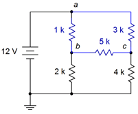
Figure 6.7.3 : Circuit for Example 6.7.1 .
This circuit uses a five resistor bridge which cannot be further simplified using basic series-parallel combinations. As a result, the techniques presented in Chapter 5 will not be sufficient to obtain a solution. A delta-Y conversion is proposed to simplify the circuit instead. We begin by defining a delta configuration using the top three resistors (shown in blue). When replaced with a Y configuration, we will have resistors in series with the 2 k\( \Omega \) and 4 k\( \Omega \), and a third resistor in series with the source. This new network can solved using basic series-parallel techniques.
Note that a Y-delta is not as good of a choice. For example, using the 1 k\( \Omega \), 2 k\( \Omega \) and the 5k\( \Omega \) as a sideways Y, the delta version leaves resistors in parallel with the 3 k\( \Omega \) and the 4 k\( \Omega \), and another in parallel with the source. This is straightforward to solve, but unfortunately, node \(b\) disappears in the process.
We shall use Equations \ref{6.4}, \ref{6.5} and \ref{6.6} to perform the delta-Y conversion. The orientation in Figure 6.7.3 is skewed compared to the reference of Figure 6.7.1 . To make them match, imagine rotating the networks of Figure 6.7.1 slightly clockwise so that point X is at the very top (matching node \(a\)), leaving Y and Z at the bottom (matching \(c\) and \(b\), respectively). Given this new orientation, \(R_a\) is the 3 k\( \Omega \), \(R_b\) is the 1 k\( \Omega \) and \(R_c\) is the 5 k\( \Omega \).
\[R_d = \frac{R_a R_b}{R_a+R_b+R_c} \nonumber \]
\[R_d = \frac{3k \Omega 1 k \Omega }{3 k \Omega +1 k \Omega +5k \Omega } \nonumber \]
\[R_d \approx 333.333 \Omega \nonumber \]
\[R_e = \frac{R_a R_c}{R_a+R_b+R_c} \nonumber \]
\[R_e = \frac{3 k \Omega 5k \Omega }{3k \Omega +1k \Omega +5k \Omega } \nonumber \]
\[R_e \approx 1.666667 k \Omega \nonumber \]
\[R_f = \frac{R_b R_c}{R_a+R_b+R_c} \nonumber \]
\[R_f = \frac{1 k \Omega 5k \Omega }{3 k \Omega +1 k \Omega +5 k \Omega } \nonumber \]
\[R_f \approx 555.556 \Omega \nonumber \]
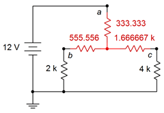
Figure 6.7.4 : Equivalent for the circuit of Figure 6.7.3 .
The equivalent network is placed back into the original circuit as shown in Figure 6.7.4 (red replaces blue). We now have a 333.333 \( \Omega \) in series with 2.555556 k\( \Omega \) \(||\) 5.666667 k\( \Omega \). To determine \(V_b\) and \(V_c\) the total equivalent resistance can be used to find the source current. From there, a current divider may be employed along with Ohm's law to find the node voltages.
\[R_{Total} = 333.333 \Omega +2.555556 k \Omega ||5.666667 k \Omega \nonumber \]
\[R_{Total} \approx 2.0946 k \Omega \nonumber \]
\[I_s = \frac{E}{R_{Total}} \nonumber \]
\[I_s \approx \frac{12 V}{2.0946 k \Omega } \nonumber \]
\[I_s \approx 5.729mA \nonumber \]
\[I_b = I_s \frac{R_{right}}{R_{left}+R_{right}} \nonumber \]
\[I_b \approx 5.729mA \frac{5.666667 k \Omega }{2.555556 k \Omega +5.666667 k \Omega } \nonumber \]
\[I_b \approx 3.9484 mA \nonumber \]
\[V_b = I_b \times R \nonumber \]
\[V_b \approx 3.948mA \times 2k \Omega \nonumber \]
\[V_b \approx 7.8968V \nonumber \]
By similar process, \(V_c\) is approximately 7.1226 volts.
To verify the results of Example 6.7.1 , we can take the two node voltages, apply them back to the original circuit, and determine whether or not they satisfy KVL or KCL.
For example, examining node \(b\), the current flowing through the 1 k\( \Omega \) resistor has to equal the sum of the currents flowing through the 2 k\( \Omega \) and 5 k\( \Omega \) resistors, via KCL.
\[I_{1k} = \frac{V_a−V_b}{R} \nonumber \]
\[I_{1k} \approx \frac{12 V−7.8968V}{1k \Omega } \nonumber \]
\[I_{1k} \approx 4.1032 mA \nonumber \]
\[I_{5k} = \frac{V_b−V_c}{R} \nonumber \]
\[I_{5k} \approx \frac{7.8968 V−7.1226 V}{5 k \Omega } \nonumber \]
\[I_{5k} \approx 0.1548mA \nonumber \]
\[I_{2k} = I_{1k} −I_{5k} \nonumber \]
\[I_{2k} \approx 4.1032 mA −0.1548mA \nonumber \]
\[I_{2k} \approx 3.9484 mA \nonumber \]
This result matches the current \(I_b\) calculated previously. For completeness sake, the process can be replicated for node \(c\).
Computer Simulation
For further verification, both the original circuit of Figure 6.7.3 and the converted circuit of Figure 6.7.4 are entered into a simulator, as shown in Figure 6.7.5 .
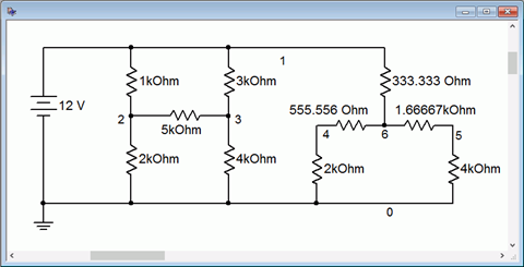
Figure 6.7.5 : Original and converted bridge circuits in simulator.
Both resistive networks are connected to a common power supply. Nodes 2 and 4 correspond to \(V_b\), while nodes 3 and 5 correspond to \(V_c\). The results of a DC operating point simulation are shown in Figure 6.7.6 .
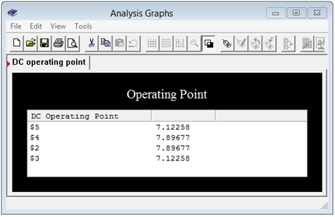
Figure 6.7.6 : Simulation results for original and converted bridges.
The voltages match each other perfectly, along with the manual calculation. In closing, we see that it is possible to swap delta networks with Y networks, and achieve identical results.
References
1In some sources the capital Greek letter delta (\(\Delta\)) is used instead of spelling out “delta” and the letter Y is spelled out as “wye”. Thus, you may come across discussion of “\(\Delta\)-Y ”, “\(\Delta\)-wye” or “delta-wye” networks. It's all the same stuff.