
5.4: Dependent Sources
- Page ID
- 52920

A dependent source is a current or voltage source whose value is not fixed (i.e., independent) but rather which depends on some other circuit current or voltage. The general form for the value of a dependent source is \(Y = kX\) where \(X\) and \(Y\) are currents and/or voltages and \(k\) is the proportionality factor. For example, the value of a dependent voltage source may be a function of a current, so instead of the source being equal to, say, 10 volts, it could be equal to twenty times the current passing through a particular resistor, or \(V=20I\).
There are four possible dependent sources: the voltage-controlled voltage source (VCVS), the current-controlled voltage source (CCVS), the voltage-controlled current source (VCCS), and the current-controlled current source (CCCS). The source and control parameters are the same for both the VCVS and the CCCS so \(k\) is unitless (although it may be given as volts/volt and amps/amp, respectively). For the VCCS and CCVS, \(k\) has units of amps/volt and volts/amp, respectively. These are referred to as the transresistance and transconductance of the sources with units of ohms and siemens.
The schematic symbols for dependent or controlled sources are usually drawn using a diamond. Also, there may be a secondary connection for the controlling current or voltage. Examples of a voltage-controlled voltage source, current-controlled voltage source, voltage-controlled current source and a current-controlled current source are shown in Figure 7.4.1 , left-to-right. On each of these symbols, the control element is shown to the left of the source. This portion is not always drawn on a schematic. Instead, the source simply may be labeled as a function, for example, \(V = 0.02 I_X\) where \(I_X\) is the controlling current.
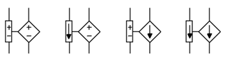
Figure 7.4.1 : Dependent sources (L to R): VCVS, CCVS, VCCS, CCCS.
Dependent sources are not “off-the-shelf” items in the same way that a battery is. Rather, dependent sources usually are used to model the behavior of more complex devices. For example, a bipolar junction transistor commonly is modeled as a CCCS while a field effect transistor may be modeled as a VCCS1. Similarly, many op amp circuits are modeled as VCVS systems. Solutions for circuits using dependent sources follow along the lines of those established for independent sources (i.e., the application of Ohm's law, KVL, KCL, etc.), however, the sources are now dependent on the remainder of the circuit which tends to complicate the analysis.
In general, there are two possible configurations: isolated and coupled. A example of the isolated form is shown in Figure 7.4.2 .
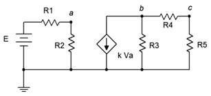
Figure 7.4.2 : Dependent source: isolated configuration.
In this configuration, the dependent source (center) does not interact with the subcircuit on the left driven by the independent source, thus it can be analyzed as two separate circuits. Solutions for this form are relatively straightforward in that the control value for the dependent source can be computed directly. This value is then substituted into the dependent source and the analysis continues as is usual. Sometimes it is convenient if the solution for a particular voltage or current is defined in terms of the control parameter rather than as a specific value (e.g., the voltage across a particular resistor might be expressed as 8 \(V_A\) instead of 12 volts, where \(V_A\) is 1.5 volts).
The second type of circuit (coupled) is somewhat more complex in that the dependent source can affect the parameter that controls the dependent source. In other words, the dependent source(s) will contribute terms that include the controlling parameter(s), thus partly controlling itself. Some additional effort will be in order to solve these circuits. To illustrate, consider the circuit of Figure 7.4.3 .
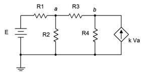
Figure 7.4.3 : Dependent source: coupled configuration.
In this example it should be obvious that the current from the dependent source can affect the voltage at node \(a\), and it is this very voltage that in turn sets up the value of the current source. Circuits of this type can be analyzed using mesh or nodal analysis. Nodal analysis works well here and is illustrated following.
We begin by defining current directions. Assume that the currents through \(R_1\) and \(R_3\) are flowing into node \(a\), the current through \(R_2\) is flowing out of node \(a\), and the current through \(R_4\) is flowing out of node \(b\). We shall number the branch currents to reflect the associated resistor. The resulting KCL equations are:
\[\sum I_{in} = \sum I_{out} \nonumber \]
\[\text{Node } a: I_1+I_3 = I_2 \nonumber \]
\[\text{Node } b: k V_a = I_3+I_4 \nonumber \]
The currents are then described by their Ohm's law equivalents:
\[\text{Node } a: \frac{E−V_a}{R_1} + \frac{V_b−V_a}{R_3} = \frac{V_a}{R_2} \nonumber \]
\[\text{Node } b: k V_a = \frac{V_b−V_a}{R_2} + \frac{V_b}{R_4} \nonumber \]
Expanding terms yields:
\[\text{Node } a: \frac{E}{R_1} − \frac{V_a}{R_1} + \frac{V_b}{R_3} − \frac{V_a}{R_3} = \frac{V_a}{R_2} \nonumber \]
\[\text{Node } b: k V_a = \frac{V_b}{R_2} − \frac{V_a}{R_2} + \frac{V_b}{R_4} \nonumber \]
Collecting terms and simplifying yields:
\[\text{Node } a : \frac{E}{R_1} = \left( \frac{1}{R_1} + \frac{1}{R_2} + \frac{1}{R_3} \right) V_a − \frac{1}{R_3} V_b \nonumber \]
\[\text{Node } b: 0 = − \left( k+ \frac{1}{R_2} \right) V_a + \left( \frac{1}{R_2} + \frac{1}{R_4} \right) V_b \nonumber \]
Values for the resistors, \(k\), and \(E\) normally are known, so the analysis proceeds directly.
Also, it is worth remembering that it is possible to perform source conversions on dependent sources, within limits. The same procedure is followed as for independent sources. The new source will remain a dependent source (e.g., converting VCVS to VCCS). This process is not applicable if the control parameter directly involves the internal impedance (i.e., is its voltage or current).
Time for an example, this one utilizing a simplified model of a transistor amplifier.
Find \(V_b\) and \(V_c\) for the circuit of Figure 7.4.4 .
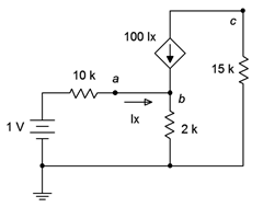
Figure 7.4.4 : Circuit for Example 7.4.1 .
This CCCS would be typical of a simple model of a bipolar junction transistor (nodes \(a\), \(b\), and \(c\)). Ideally, the output voltage, \(V_c\), would be equal to the input voltage (1 V) times the resistor ratio of 15 k\( \Omega \) / 2 k\( \Omega \) and inverted, or approximately −7.5 volts. In reality, it usually comes up a little short of this. Let's see how well this works out.
This circuit is a good candidate for nodal analysis using the general method. Note that the points labeled \(a\) and \(b\) are the same node so we can write just two KCL summations. Using the current directions as draw on the schematic, for node \(b\) we have:
\[\sum I_{in} = \sum I_{out} \nonumber \]
\[I_x+100 I_x = \frac{V_b}{2 k \Omega} \nonumber \]
\[101 \frac{1V−V_b}{10 k \Omega} = \frac{V_b}{2 k \Omega} \nonumber \]
\[10.1 mA = \left( \frac{1}{2 k \Omega} + \frac{101}{10 k \Omega} \right) V_b \nonumber \]
\[10.1 mA = 10.6 mS V_b \nonumber \]
\[V_b = 0.95283 V \nonumber \]
For node \(c\) we have:
\[\sum I in = \sum I out \nonumber \]
\[− \frac{V_c}{15 k \Omega} = 100 I_x \nonumber \]
\[− \frac{V_c}{15 k \Omega} = 100 \frac{1V−V_b}{10 k \Omega} \nonumber \]
\[V_c = −7.0755 V \nonumber \]
Alternately, instead of writing the second KCL summation we could have used \(V_b\) to determine \(I_x\), i.e., \((1 − V_b)/10\) k\( \Omega \). As the current through the 15 k\( \Omega \) resistor is \(100 I_x\), we could then use Ohm's law to find \(V_c\). In any case, we do see that \(V_c\) is inverted and just shy of the 7.5 volt estimate.
Computer Simulation
For verification, the dependent source circuit of Example 7.4.1 is entered into a simulator as shown in Figure 7.4.5 . A DC operating point analysis is run, the results of which are shown in Figure 7.4.6 . The output voltage shows roughly −7.08 volts and a \(V_b\) of just under 1 volt, thus achieving excellent agreement with the manual calculation.
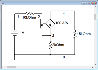
Figure 7.4.5 : Circuit of Figure 7.4.4 in a simulator.
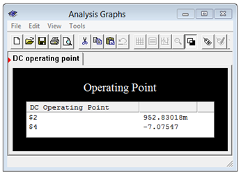
Figure 7.4.6 : Simulation results for the circuit of Figure 7.4.4 .
While this simulation is effective in this case, just using a dependent source to stand in for a transistor is rather limited. There are many other, perhaps more subtle, elements to a proper transistor model that will ensure both greater accuracy and proper results under a wide range of operating conditions. Any quality simulator will include a parts library using simulation models that are fine-tuned to particular manufacturer part numbers.
References
1For details, see Fiore, J.M., Semiconductor Devices: Theory and Application, and Operational Amplifiers and Linear Integrated Circuits: Theory and Application, both free OER titles.