
12.3: Superposition Theorem
- Page ID
- 52970

Superposition allows the analysis of multi-source AC series-parallel circuits. Superposition can only be applied to networks that are linear and bilateral. Fortunately, all of components we have discussed; resistors, capacitors and inductors, fall into that category. Further, superposition cannot be used to find values for non-linear functions, such as power, directly. This is not a limitation though because power can be computed from the resulting voltage or current values.
The basic idea is to determine the contribution of each source by itself, and then combine the results to get the final answer. The contributions are either all voltages or all currents, depending on need. We can state the superposition theorem as:
Theorem \(\PageIndex{1}\): Superposition Theorem
Any voltage or current in a multi-source linear bilateral network may be determined by summing the contributions caused by each source acting alone, with all other source replaced by their internal impedance.
The process generates a series of new single-source circuits, one for each source. These new circuits are then analyzed for the parameter(s) of interest.
Consider the circuit depicted in Figure \(\PageIndex{1}\).
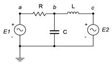
Here we see two voltage sources, \(E1\) and \(E2\), driving a three element series-parallel network. As there are two sources, two derived circuits must be created; one using only \(E1\) and the other using only \(E2\). When considering a given source, all other sources are replaced by their ideal internal impedance: for a voltage source, that's a short; and for a current source, an open. We start by considering \(E1\). In the new circuit \(E2\) is replaced with a short. This leaves a fairly simple network where \(X_C\) and \(X_L\) are in parallel. This combination is in series with \(R\) and \(E1\). Using basic series-parallel techniques, we can solve for desired quantities such as the current flowing through \(R\) or the voltage \(v_b\). It is important to indicate the reference current direction and voltage polarity with respect to the source being considered (here, that's left-to-right and positive, respectively). The process is then repeated for \(E2\), shorting \(E1\) and leaving us with \(R\) in parallel with \(X_C\), which is in turn in series with \(X_L\) and \(E2\). Note that although in this version \(V_b\) is still positive, the reference current direction for \(R\) is now right-to-left. The numerical results from this version are added to those of the \(E1\) version (minding polarities and directions) to achieve the final result. If power is needed, it can be computed from these currents or voltages. Note that superposition can work with a mix of current sources and voltage sources. The practical downside is that for large circuits using many sources, numerous derived circuits will need to be analyzed. For example, if there are three voltage sources and two current sources, then a total of five derived circuits will be created.
It is also possible to use superposition to find the resulting currents or voltages in a circuit that uses sources with different frequencies. In this instance, the equivalent circuits will have different reactance values. In fact, a single non-sinusoidal source can be analyzed using this method by treating the source as a series of superimposed sine waves with each sine source producing a new circuit with its own unique reactance values.
To summarize the superposition technique:
- For every voltage or current source in the original circuit, create a new sub-circuit. The sub-circuits will be identical to the original except that all sources other than the one under consideration will be replaced by their ideal internal impedance. This means that all remaining voltage sources will be shorted and all remaining current sources will be opened.
- Indicate the reference current directions and voltage polarities on each of the new sub-circuits, as generated by the source under consideration.
- Solve each of the sub-circuits for the desired voltages and/or currents using standard series-parallel analysis techniques. Make sure to note the reference voltage polarities and current directions for these items.
- Add all of the contributions from each of the sub-circuits to arrive at the final values, being sure to account for current directions and voltage polarities in the process.
To illustrate the superposition technique, let's reexamine the the dual source circuit shown in Figure 5.2.12 (repeated in Figure \(\PageIndex{2}\) for ease of reference). We will solve this using superposition and compare the results to those of Example 5.2.3 which used source conversion.
Example \(\PageIndex{1}\)
For the circuit of Figure \(\PageIndex{2}\), determine \(v_b\) using superposition. \(I = 2E−3\angle 90^{\circ}\) amps peak and \(E = 10\angle 0^{\circ}\) volts peak.
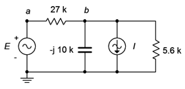
As the circuit has two sources, it will require two sub-circuits. For the voltage source, the current source will be replaced with an open. For the second circuit utilizing the current source, the voltage source will be replaced with a short. First, using the voltage source we find:
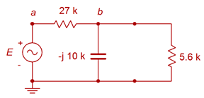
For this circuit, \(v_b\) may be determined via a voltage divider. To proceed, we need the impedance of the parallel combo on the right.
\[Z_{right2} = \frac{R\times jX_C}{R − jX_C} \nonumber \]
\[Z_{right2} = \frac{5.6 k\Omega \times (− j 10 k\Omega )}{5.6 k\Omega − j 2k \Omega} \nonumber \]
\[Z_{right2} = 4886\angle −29.2^{\circ} \Omega \nonumber \]
Now for the voltage divider to find the contribution of the first source to \(v_b\).
\[v_{b1} = E \frac{Z_{right2}}{Z_{right2} + R_1} \nonumber \]
\[v_{b1} = 10 \angle 0^{\circ} V \frac{4886\angle −29.2^{\circ} \Omega}{4886\angle −29.2^{\circ} \Omega +27 k \Omega} \nonumber \]
\[v_{b1} = 1.558\angle −24.88^{\circ} V \nonumber \]
We turn our attention to the current source's contribution. We short the voltage source and redraw:
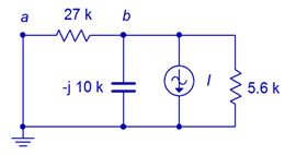
This is a simple parallel circuit. We can find \(v_b\) by placing the resistors and capacitors in parallel, and then using Ohm's law. Note that the reference direction of the current source is downward, meaning that the component current is upward, which makes \(v_b\) negative (i.e., + to − bottom to top). The parallel impedance is:
\[Z_{total} = \frac{1}{\frac{1}{X_C} + \frac{1}{R_1} + \frac{1}{R_2}} \nonumber \]
\[Z_{total} = \frac{1}{\frac{1}{− j 10 k\Omega} + \frac{1}{27k \Omega} + \frac{1}{5.6k \Omega}} \nonumber \]
\[Z_{total} = 4208\angle −24.9 ^{\circ} \Omega \nonumber \]
We apply Ohm's law to find this source's contribution to \(v_b\).
\[v_{b2} = I\times Z_{total} \nonumber \]
\[v_{b2} =−2E-3\angle 90^{\circ} A\times 4208\angle −24.9^{\circ} \Omega \nonumber \]
\[v_{b2} = 8.416\angle −114.9^{\circ} V \nonumber \]
The final result is the sum of the two parts:
\[v_b = v_{b1} +v_{b2} \nonumber \]
\[v_b = 1.558\angle −24.88^{\circ} V +8.416\angle −114.9 ^{\circ} V \nonumber \]
\[v_b = 8.558\angle −104.4 ^{\circ} V \nonumber \]
This is virtually the same value obtained using the source conversion technique in the prior example.
As mentioned previously, superposition can be used to determine the results even when the sources use different frequencies. This will be explored in the next example.
Example \(\PageIndex{2}\)
For the circuit of Figure \(\PageIndex{5}\), determine \(v_b\).
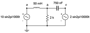
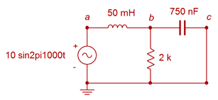
Using superposition, we derive two new circuits, each with unique reactance values. The first circuit is shown in Figure \(\PageIndex{6}\).
The reactance values are:
\[X_L = j 2\pi f L \nonumber \]
\[X_L = j 2\pi 1kHz 50mH \nonumber \]
\[X_L\approx j 314.2\Omega \nonumber \]
\[X_C =− j \frac{1}{2 \pi f C} \nonumber \]
\[X_C =− j \frac{1}{2 \pi 1kHz 750 nF } \nonumber \]
\[X_C \approx − j 212.2\Omega \nonumber \]
A voltage divider can be used to find this portion of \(v_b\). The parallel combo of the 2 k\(\Omega\) resistor and capacitor is \(211\angle −83.9^{\circ} \Omega\).
\[v_{b1} = E \frac{Z_{right2}}{Z_{right2} + X_L} \nonumber \]
\[v_{b1} = 10 \angle 0^{\circ} V \frac{211\angle −83.9^{\circ} \Omega}{211\angle −83.9^{\circ} \Omega +314.2\angle 90 ^{\circ} \Omega} \nonumber \]
\[v_{b1} = 19.78\angle −161.9 ^{\circ} V \nonumber \]
Remember, this waveform is at a frequency of 1 kHz. We can repeat this process for the second source which uses 10 kHz. At this new frequency the inductive reactance will be ten times larger, or \(j3142 \Omega\), and the capacitive reactance will be ten times smaller, or \(−j21.22 \Omega\). The new circuit is shown in Figure \(\PageIndex{7}\).
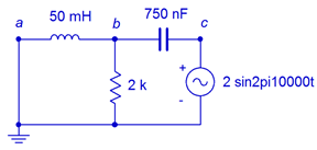
Once again, a voltage divider can be used to find this portion of \(v_b\). The parallel combo of the 2 k\(\Omega\) resistor and inductor is \(1687\angle 32.5^{\circ} \Omega\).
\[v_{b2} = E \frac{Z_{left2}}{Z_{left2} + X_C} \nonumber \]
\[v_{b2} = 2\angle 0^{\circ} V \frac{1687\angle 32.5^{\circ} \Omega}{1687\angle 32.5^{\circ} \Omega +21.22\angle −90^{\circ} \Omega} \nonumber \]
\[v_{b2} = 2.01\angle 0.6^{\circ} V \nonumber \]
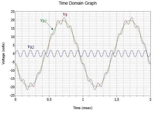
This contribution is at a frequency of 10 kHz. Thus, the combination is a relatively small 10 kHz sine at about 2 volts peak riding on a 1 kHz sine that is nearly ten times larger in amplitude. This is shown in Figure \(\PageIndex{8}\).
Computer Simulation
In order to verify the two-component waveform of Example \(\PageIndex{2}\), the circuit of Figure \(\PageIndex{5}\) is captured in a simulator as shown in Figure \(\PageIndex{9}\).
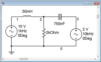
A transient analysis is performed. The results are illustrated in Figure \(\PageIndex{10}\).
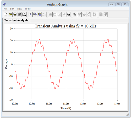
The results match the computed values nicely. We can see the small amplitude high frequency sine wave effectively following the contour of the much larger 1 kHz sine wave.