
12.2: Source Conversions
- Page ID
- 52969

In DC analysis, we noted that real world sources have practical limits: voltage sources cannot produce infinite current and current sources cannot produce infinite voltage. A simple way of creating a more accurate model for independent sources is to include an internal resistance. For DC voltage sources, a resistance is added in series with the source, and for DC current sources a resistance is added in parallel with the source. While this works well enough for typical DC sources, the AC situation is a little more complicated.
Models for AC Sources
Just as we added a simple resistance to the DC sources to make improved models, we can add a complex impedance to AC sources to do likewise. Once again, it is possible to make even more involved models that will be more accurate, but for most work, this addition will suffice. Generally, there are wider variations in values for the AC case than the DC case.
We can think of AC sources as belonging in one of two broad categories. First, there are power generators, that is, systems designed to generate and deliver power for other electrical devices. This would include the AC mains system in a residence or a portable power generator. At the other end of the spectrum are signal sources such as transducers and sensors. These devices are generally low power and are not designed to produce particularly high currents, quite the opposite of generators.
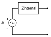
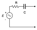
The model for an AC voltage source adds an impedance in series, as shown in Figure \(\PageIndex{1}\). This impedance sets an upper limit on the source's current output. Even if the output terminals are shorted, the maximum current will be dictated via Ohm's law to be the source voltage divided by the internal impedance, or \(E/Z_{internal}\). Obviously, this internal impedance will create some voltage divider effect with the attached load. To minimize this effect, the impedance should be as small as practicably possible. Thus,
\[\text{The ideal internal impedance of a voltage source is zero ohms (a short).} \nonumber \]
It is not always possible to get close to this ideal. In fact, in some situations the AC source is far removed from the ideal.
Consider the signal source shown in Figure \(\PageIndex{2}\). This is a pickup for an electric bass guitar. This device is used to translate the motions of guitar strings into a voltage that can be fed to an amplifier. It consists of a few thousand turns of very fine magnet wire wrapped around a magnet.
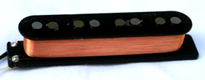
When the metal guitar strings vibrate, they alter the surrounding magnetic field. As the magnetic field changes, it induces a current, and hence a voltage, in the coil. The resulting signal is an electrical analog of the string vibrations. It is, quite literally, an AC signal source. But what of its internal impedance? The coil is made of wire between AWG 40 and 45, and may be in excess of 1000 feet (300 meters) in length. Consulting an AWG table1, we find that this will yield 1000 or more ohms of resistance. Of course, a few thousand turns of wire will also create a hefty inductance and pickups such as this may exhibit an inductance of a few henries. Putting these pieces together, the equivalent internal impedance might look something like that shown in Figure 5.3.
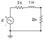
Clearly, values like these are a far cry from the fractional ohm values found in power generation sources, and they present unique challenges. In the circuit of Figure \(\PageIndex{3}\), the component labeled \(Z_{in}\) represents the input impedance of the associated amplifier. Typically, it would be highly resistive but the magnitude can vary quite a bit depending on the application. A guitar or bass amplifier may exhibit 1 M\(\Omega\) or more, while an auxiliary input on a home stereo might be 10 k\(\Omega\). What happens if you plug a guitar into your hi-fi? Obviously, this system creates a voltage divider between the internal impedance of the pickup and the input impedance of the amplifier, but more importantly, the divider is a function of frequency. At low frequencies like 100 Hz, the inductive reactance is small, around \(j600 \Omega \), and the signal loss to a 10 k\(\Omega\) input is not that great. On the other hand, at a high frequency such as 10 kHz, the inductive reactance will be over \(j60 k\Omega \) resulting in considerable signal loss. Thus, the high frequencies are reduced relative to the low frequencies. The sonic effect is akin to turning down the treble control — everything will seem muffled. If the input impedance is increased considerably, say by a factor of 100, then the voltage divider effect at all audible frequencies will be negligible and the the instrument will sound true to form. Finally, although this example shows a substantial inductance, it is possible for AC sources to have an associated capacitance, or even have negligible reactance (i.e., be purely resistive).
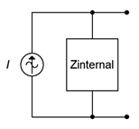
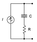
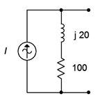
For a current source, the improved model adds an impedance in parallel, as shown in Figure \(\PageIndex{4}\). This impedance sets an upper limit on the source's voltage output. If the output terminals are opened, the maximum voltage will no longer produce a huge voltage. Instead, it is dictated by Ohm's law to be the source current times the internal impedance, or \(I\cdot Z_{internal}\). This internal impedance will create some current divider effect with the attached load. To minimize this effect, the internal impedance should be as large as practicably possible. Thus,
\[\text{The ideal internal impedance of a current source is infinite ohms.} \nonumber \]
From here on, whenever we deal with practical voltage and current sources, we understand that these sources have some associated internal resistance, even if they're not shown explicitly in a schematic diagram. Further, whenever we talk about ideal sources, we simply use a short for the internal impedance of a voltage source and an open for the internal impedance of a current source.
Source Equivalences
For any voltage source consisting of an ideal voltage source with a series internal impedance, an equivalent current source may be created. Similarly, for any current source consisting of an ideal current source with a parallel internal impedance, an equivalent voltage source may be created. By “equivalent”, we mean that both circuits will produce the same voltage and current to identical loads. Consider the simple voltage source on the left side of Figure \(\PageIndex{5}\). Its equivalent current source is shown on the right.
For reasons that will become apparent under the section on Thévenin's theorem following, the internal impedances of these two circuits must be identical if they are to behave identically. Knowing that, it is a straightforward process to find the required values of the other source. The current/voltage characteristic is linear for these circuits, and a straight plot line can be defined by just two points. The two obvious points to use are the opened and shorted load cases. In other words, if the circuit is equivalent for these two situations, it must work for any load. The shorted load case produces a large load current with zero load voltage, and the opened load case produces a large load voltage with zero load current. It would not make sense if the equivalent source could produce a greater current or voltage under the same extreme conditions as the original.
For example, given a voltage source, the current that can be developed when the load is shorted is \(E/Z_{internal}\). Under that same load condition, all of the current from the current source version must be flowing through the load (otherwise the load isn't shorted). Therefore, the value of the equivalent current source must be the current of \(E/Z_{internal}\). Note that the resulting source normally will not have the same phase angle as the original source due to the phase angle of the associated impedance.
To continue, if we look at the open load case for the voltage source, the load current would be zero and the load voltage would be the entire source voltage of \(E\). For the current source, the load would also see no current and its voltage would be the voltage appearing across its internal resistance which is \(Z_{internal}\) times the current \(E/Z_{internal}\), or just \(E\). Thus, the two behave identically at the load limits.
Similarly, if we start with a current source, an open load produces a load voltage of \(I\cdot Z_{internal}\). Therefore, the equivalent voltage source must have a value of \(I\cdot Z_{internal}\). For the current source, a shorted load would produce a load current equal to the source value, or \(I\). The voltage source version would produce a current of \(E/Z_{internal}\), where the value of \(E\) was just found to be equal to \(I\cdot Z_{internal}\), and thus the load current would be \(I\cdot Z_{internal}/Z_{internal}\), or just \(I\). Once again, the two versions behave identically at the load limits.
Changing the source frequency results in different values for both the reactance and the converted source voltage or current, thus the equivalent is valid only for the frequency in question.
To summarize the process of source conversion:
- The internal impedance will be the same for both versions.
- If converting from a voltage source to a current source, the value of the current source will be the short circuit current available from the voltage source (i.e., shorted load case), and is equal to \(E/Z_{internal}\).
- If converting from a current source to a voltage source, the value of the voltage source will be the open circuit voltage available from the current source (i.e., opened load case), and is equal to \(I\cdot Z_{internal}\).
- The equivalent is unique to the frequency of the source.
If a multi-source is being converted (i.e., voltage sources in series or current sources in parallel), first combine the sources to arrive at the simplest source and then do the conversion. Do not convert the sources first and then try to combine them as you will wind up with series-parallel configurations rather than simple sources.
Judicious use of source conversions can sometimes simplify multi-source circuits by allowing converted sources to be combined, resulting in a single source.
Example \(\PageIndex{1}\)
Convert the source of Figure \(\PageIndex{6}\) into its current source equivalent. \(E = 2 \angle 0^{\circ}\) volts RMS.
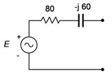
First, the existing impedance of \(80 − j60 \Omega\) does not change, it is simply moved to a parallel position. To find the value of the current source, compute the short circuit current the existing source is capable of producing.
\[I = \frac{E}{Z} \nonumber \]
\[I = \frac{2\angle 0^{\circ} V}{80 − j 60\Omega} \nonumber \]
\[I = 0.02\angle 36.9^{\circ} A \nonumber \]
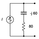
The result is shown in Figure \(\PageIndex{7}\). The current source is 20 mA RMS with a leading phase angle of 36.9 degrees.
Example \(\PageIndex{2}\)
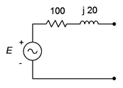
Convert the source of Figure \(\PageIndex{8}\) into its voltage source equivalent. \(I = 0.1\angle 0^{\circ}\)amps peak.
Again, the internal impedance of \(100 + j20 \Omega\) does not change and we simply place it in series. To find the value of the voltage source, find the open circuit voltage the existing source is capable of producing.
\[E = I\times Z \nonumber \]
\[E = 0.1\angle 0^{\circ} A\times (100 +j 20\Omega ) \nonumber \]
\[E \approx 10.2 \angle 11.3^{\circ} V \nonumber \]
The equivalent is shown in Figure \(\PageIndex{9}\). The voltage source \(E\) is 10.2 volts peak with a leading phase angle of 11.3 degrees.
Computer Simulation
To verify this process, the circuits of Figures \(\PageIndex{8}\) and \(\PageIndex{9}\) are entered into a simulator. The original circuit simply specified an inductive reactance so a convenient frequency of 1 kHz was used and then an appropriate inductor was created that would yield the desired reactance of \(j20 \Omega\). This turned out to 3.183 mH. Further, a random load resistor (200 \(\Omega\)) was picked and applied to both circuits. The result is shown in Figure 5.10.
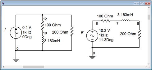
If these two circuits are equivalent, then the voltages seen across the 200 \(\Omega\) load resistors should be identical. These voltages correspond to node voltages 12 and 8. A quick voltage divider computation shows that the load voltage should be approximately \(6.785\angle 7.5^{\circ}\) volts peak.
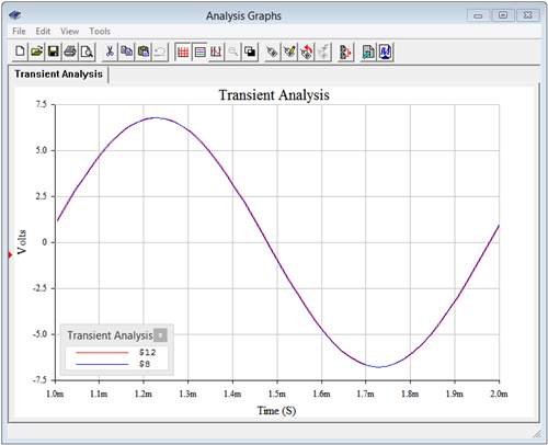
A transient analysis is performed, plotting the load voltages. The results are shown in Figure \(\PageIndex{11}\). The plot itself is delayed by one millisecond in order to get past the initial turn-on transient. Further, the current source circuit is shifted by approximately 2 microseconds. Without this slight shift in time, the two voltages perfectly overlap so that it appears there is only one trace. By looking carefully at the graph it can be seen that there are indeed two traces. The amplitudes of these waveforms match each other perfectly and also match the computed result.
Now let's turn our attention to using source conversion to simplify and solve a multisource circuit.
Example \(\PageIndex{3}\)
For the circuit of Figure \(\PageIndex{12}\), determine \(v_b\). \(I = 2E−3\angle 90^{\circ}\) amps peak and \(E = 10\angle 0^{\circ}\) volts peak.
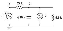
One method of solution is to transform the voltage source into a current source. By doing so, the entire circuit is reduced to a parallel network. The two current sources can then be summed and the remaining three components can be combined into one equivalent parallel impedance. At that point Ohm's law can be used to find \(v_b\).
The value of the current source is:
\[I_c = \frac{E}{Z} \nonumber \]
\[I_c = \frac{10\angle 0^{\circ} V}{27 k \Omega} \nonumber \]
\[I_c = 0.3704E-3\angle 0^{\circ} A \nonumber \]
The converted circuit is shown in Figure \(\PageIndex{13}\) (in blue).
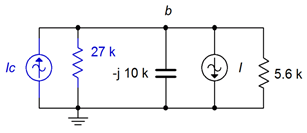
Combining the two current sources and using an upward reference direction yields:
\[I_{total} = I_c−I \nonumber \]
\[I_{total} = 0.3704E-3\angle 0^{\circ} A−2E-3\angle 90^{\circ} A \nonumber \]
\[I_{total} = 2.034E-3\angle −79.5^{\circ} A \nonumber \]
The combined impedance is:
\[Z_{total} = \frac{1}{\frac{1}{X_C} + \frac{1}{R_1} + \frac{1}{R_2}} \nonumber \]
\[Z_{total} = \frac{1}{\frac{1}{− j 10 k\Omega} + \frac{1}{27k \Omega} + \frac{1}{5.6k \Omega}} \nonumber \]
\[Z_{total} = 4208\angle −24.9 ^{\circ} \Omega \nonumber \]
And finally we compute \(v_b\):
\[v_b = I_{total} \times Z_{total} \nonumber \]
\[v_b = 2.034E-3\angle −79.5^{\circ} A\times 4208\angle −24.9^{\circ} \Omega \nonumber \]
\[v_b = 8.56\angle −104.4 ^{\circ} V \nonumber \]
We can perform a KCL crosscheck at node \(b\) to verify the results in the original circuit. Given the reference directions, all currents are flowing out of the node except for the current supplied by the voltage source.
\[i_{Esource} = \frac{E−v_b}{R_1} \nonumber \]
\[i_{Esource} = \frac{10\angle 0^{\circ} V−8.56\angle −104.4 ^{\circ} V}{27 k\Omega} \nonumber \]
\[i_{Esource} = 0.544E-3\angle 34.4^{\circ} A \nonumber \]
The remaining three currents should add up to this value.
\[i_{capacitor} = \frac{v_b}{X_C} \nonumber \]
\[i_{capacitor} = \frac{8.56 \angle −104.4 ^{\circ} V}{− j 10 k\Omega} \nonumber \]
\[i_{capacitor} = 0.856E-3\angle −14.4^{\circ} A \nonumber \]
\[i_{R2} = \frac{v_b}{R_2} \nonumber \]
\[i_{R2} = \frac{8.56 \angle −104.4 ^{\circ} V}{5.6k \Omega} \nonumber \]
\[i_{R2} = 1.53E-3\angle −104.4^{\circ} A \nonumber \]
Finally, \(0.856E−3\angle −14.4^{\circ} + 1.53E−3\angle −104.4^{\circ} + 2E−3\angle 90^{\circ}\) amps does indeed equal \(0.544E−3\angle 34.4^{\circ}\) amps, within carried rounding error.
References
1Such as the one found in Chapter 2 of the companion text, DC Electrical Circuit Analysis, a companion free OER text by the author.