
12.6: Advanced Topic- Delta-Y (Pi-T) Conversions
- Page ID
- 52973

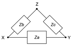
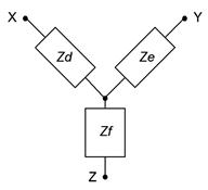
Certain component configurations, such as bridged networks, cannot be reduced to a single impedance using basic series-parallel conversion techniques. One method for simplification involves converting sections into more convenient forms. The configurations in question are networks with three external connection points. Due to the manner in which they drawn, they are referred to as delta networks and Y networks1. These configurations are shown in Figure \(\PageIndex{1}\). Note that the terminal designation of the delta version are upside down compared to those of the Y configuration.
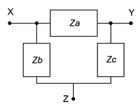
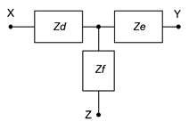
These networks can be redrawn without angles. In this form they are known as pi (also called “\(\pi\)”) networks and T (also called “tee”) networks. These configurations are shown in Figure \(\PageIndex{2}\).
It is possible to convert back and forth between delta and Y networks in many cases. That is, for a given delta network, there may exist a Y network such that the impedances seen between the X, Y and Z terminals are identical, and vice versa. Consequently, one configuration can replace another in order to simplify a larger circuit. Unlike the DC version, certain AC networks cannot be converted using the following technique (see the final Challenge problem for an investigation of this).
\(\Delta\)-Y Conversion
A true equivalent circuit would present the same impedance between any two terminals as the original circuit. Consider the circuits of Figure \(\PageIndex{1}\) for the unloaded case (i.e., just these networks with nothing else connected to them). The equivalent impedances seen between each pair of terminals for the delta and the Y respectively are:
\[Z_{XY} = Z_a || (Z_b+Z_c) = Z_d + Z_e \label{5.3} \]
\[Z_{XZ} = Z_b || (Z_a+Z_c) = Z_d + Z_f \label{5.4} \]
\[Z_{ZY} = Z_c || (Z_b+Z_a) = Z_e + Z_f \label{5.5} \]
Let's assume that we have the delta network and are looking for the Y network equivalent. We start by focusing on the final set of terms for each of the three expressions (e.g., \(Z_{XY} = Z_d + Z_e\)). Note that we have three equations with three unknowns (\(Z_d\), \(Z_e\) and \(Z_f\)). Thus, they can be solved using a term elimination process. If we subtract Equation \ref{5.5} from Equation \ref{5.3}, we can eliminate the second impedance (\(Z_e\)) and arrive at a difference between the first and third unknown impedance s (\(Z_d − Z_f\)). This quantity can then be added to Equation \ref{5.4} to eliminate the third impedance (\(Z_f\)), leaving just the first unknown impedance (\(Z_d\)).
\[(Z_d + Z_e) − (Z_e + Z_f) = (Z_d − Z_f) = Z_a || (Z_b+Z_c) − Z_b || (Z_a+Z_c) \nonumber \]
\[(Z_d + Z_f) + (Z-d − Z_f) = 2Z_d = 2( Z_b || (Z_a+Z_c) + Z_a || (Z_b+Z_c) − Z_c || (Z_a+Z_b) ) \nonumber \]
Therefore,
\[Z_d = Z_b || (Z_a+Z_c) + Z_a || (Z_b+Z_c) − Z_c || (Z_a+Z_b) \nonumber \]
which, after simplifying2, is:
\[Z_d = \frac{Z_a Z_b}{Z_a+Z_b+Z_c} \label{5.6} \]
Similarly, we can show that
\[Z_e = \frac{Z_a Z_c}{Z_a+Z_b+Z_c} \label{5.7} \]
\[Z_f = \frac{Z_bZ_c}{Z_a+Z_b+Z_c} \label{5.8} \]
Note that if the magnitudes and angles of three original impedances are identical, the magnitudes of the Y equivalent impedances will all be one-third of the original magnitude, and with the original phase angle.
Y-\(\Delta\) Conversion
For the reverse process of converting from Y to delta, start by noting the similarities of the expressions for \(Z_d\), \(Z_e\) and \(Z_f\) (i.e., Equations \ref{5.6} through \ref{5.8}). If two of these expressions are divided, a single equation for \(Z_a\), \(Z_b\) or \(Z_c\) will result. For example, using Equations \ref{5.6} and \ref{5.7}:
\[\frac{Z_d}{Z_e} = \frac{\frac{Z_a Z_b}{Z_a+Z_b+Z_c}}{\frac{Z_a Z_c}{Z_a+Z_b+Z_c}} \nonumber \]
\[\frac{Z_d}{Z_e} = \frac{Z_a}{Z_b}\frac{Z_a}{Z_c} \nonumber \]
\[\frac{Z_d}{Z_e} = \frac{Z_b}{Z_c} \nonumber \]
Therefore,
\[\frac{Z_b}{Z_c} = \frac{Z_d}{Z_e} \nonumber \]
\[Z_b = \frac{Z_c Z_d}{Z_e} \nonumber \]
This process can be repeated for Equations \ref{5.6} and \ref{5.8} to obtain an expression for \(Z_a\). The two expressions for \(Z_a\) and \(Z_b\) can then be substituted into Equation \ref{5.6} to obtain an expression for \(Z_c\) that utilizes only \(Z_d\), \(Z_e\) and \(Z_f\). A similar process is followed for \(Z_a\) and \(Z_b\) resulting in:
\[Z_a = \frac{Z_d Z_e + Z_e Z_f + Z_d Z_f}{Z_f} \label{5.9} \]
\[Z_b = \frac{Z_d Z_e+Z_e Z_f +Z_d Z_f}{Z_e} \label{5.10} \]
\[Z_c = \frac{Z_d Z_e+Z_e Z_f +Z_d Z_f}{Z_d} \label{5.11} \]
If the Y network consists of three identical impedances, then the values of the delta equivalent will all be three times the original magnitude, the inverse of the situation when converting from delta to Y.
In summation, equations \ref{5.6}, \ref{5.7} and \ref{5.8} can be used to convert a delta network into a Y network, and equations \ref{5.9}, \ref{5.10} and \ref{5.11} can be used to convert a Y network into a delta network. Examples of how to apply this technique to tame up-to-now intractable series-parallel networks follow.
Example \(\PageIndex{1}\)
Convert the network of Figure \(\PageIndex{3}\) into its delta configuration equivalent.
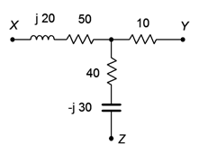
Referring back to Figure \(\PageIndex{2}\), use Equation \ref{5.9} to determine \(Z_a\).
\[Z_a = \frac{Z_d Z_e + Z_e Z_f +Z_d Z_f}{Z_f} \nonumber \]
\[Z_a = \frac{(50 +j 20\Omega )(10\Omega )+(10\Omega )(40 − j 30\Omega )+(50 +j 20\Omega )(40 − j30\Omega )}{(40 − j 30\Omega )} \nonumber \]
\[Z_a = 65.6 +j 29.2\Omega \nonumber \]
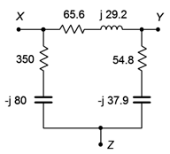
\(Z_b\) and \(Z_c\) may be determined in similar manner using Equations \ref{5.10} and \ref{5.11}:
\[Z_b = 350 − j80 \Omega \nonumber \]
\[Z_c = 54.8 − j37.9 \Omega \nonumber \]
The equivalent is shown in Figure \(\PageIndex{4}\).
Remember, a complex impedance can always be expressed in rectangular form. Rectangular form can be expressed directly as a series combination of a resistor and either an inductive or capacitive reactance. Even if the original impedances of a network are in a parallel form (or even a more complex form), the equivalent can be expressed as a series combination.
Example \(\PageIndex{2}\)
Determine \(v_a\) in the circuit of Figure \(\PageIndex{5}\). Assume the source has a phase angle of zero degrees.
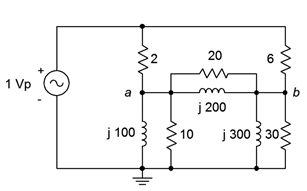
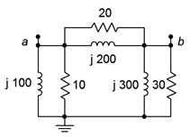
This circuit cannot be simplified sufficiently using basic series-parallel techniques due to the bridge section. The components between and below nodes \(a\) and \(b\) comprise a delta network, as shown in Figure \(\PageIndex{6}\). If this network is replaced with a Y equivalent, the resulting circuit reduces to a simple series-parallel system.
Before continuing, it would be helpful to determine the impedance of each of the parallel sections. For the leftmost pair:
\[Z_{left2} = \frac{R \times jX_L}{R +jX_L} \nonumber \]
\[Z_{left2} = \frac{10\Omega \times j 100 \Omega}{10\Omega +j 100 \Omega} \nonumber \]
\[Z_{left2} = 9.9+j 0.99\Omega \nonumber \]
In similar manner, the top pair is determined to be \(19.8 + j1.98 \Omega \) and the rightmost pair is \(29.7 + j2.97 \Omega \). Referring back to Figure \(\PageIndex{2}\), we can use Equation \ref{5.6} to determine \(Z_d\).
\[Z_d = \frac{Z_a Z_b}{Z_a + Z_b + Z_c} \nonumber \]
\[Z_d = \frac{(19.8+j 1.98\Omega ) \times (9.9+j 0.99\Omega )}{(19.8+j 1.98\Omega )+(9.9+j 0.99\Omega )+(29.7+j 2.97\Omega ) } \nonumber \]
\[Z_d = 3.3+j 0.33\Omega \nonumber \]
Likewise, we can use Equations \ref{5.7} and \ref{5.8} to determine \(Z_e\) and \(Z_f\).
\[Z_e = 9.9 + j0.99 \Omega \nonumber \]
\[Z_f = 4.95 + j0.495 \Omega \nonumber \]
Swapping the equivalent Y network into the original circuit leads us to the circuit of Figure \(\PageIndex{7}\) (Y network shown in blue). This circuit can be simplified directly to find \(v_a\).
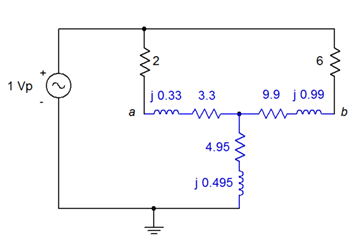
In this equivalent circuit, \(v_a\) is simply the source voltage of \(1\angle 0^{\circ}\) minus the voltage across the 2 \(\Omega\) resistor. The immediate goal, then, is to find the current through that resistor. This can be achieved via a current divider once the source current is known. To find the source current, we need to find the total impedance of the network. On the upper left side, \(Z_d\) is in series with the 2 \(\Omega\) resistor for a total of \(5.3 + j0.33 \Omega \). This is in parallel with the upper right side total of \(15.9 + j0.99 \Omega \).
\[Z_{upper} = \frac{Z_{upperleft} \times Z_{upperright}}{Z_{upperleft} +Z_{upperright}} \nonumber \]
\[Z_{upper} = \frac{(5.3 +j0.33\Omega ) \times (15.9 +j 0.99\Omega )}{(5.3 +j 0.33\Omega ) +(15.9 +j 0.99\Omega )} \nonumber \]
\[Z_{upper} = 3.975 +j 0.2475\Omega \nonumber \]
This is in series with the lower section of \(4.95 + j0.495 \Omega \) for a total of \(8.956\angle 4.76^{\circ} \Omega \). Using Ohm's law, we find the source current:
\[i_{source} = \frac{E}{Z_{total}} \nonumber \]
\[i_{source} = \frac{1\angle 0^{\circ} V}{8.956\angle 4.76^{\circ} \Omega} \nonumber \]
\[i_{source} = 0.1117\angle −4.76^{\circ} A \nonumber \]
Now for the current divider and also Ohm's law for the 2 \(\Omega\) resistor.
\[i_{2\Omega} = i_{source} \frac{Z_{upperright}}{Z_{upperright} +Z_{upperleft}} \nonumber \]
\[i_{2\Omega} = 0.1117\angle −4.76^{\circ} A \frac{15.9+j 0.99\Omega}{ (15.9+j 0.99\Omega )+(5.3+j 0.33\Omega ) } \nonumber \]
\[i_{2\Omega} = 83.7E-3\angle −4.76^{\circ} A \nonumber \]
\[v_{2\Omega} = i 2\Omega \times R \nonumber \]
\[v_{2\Omega} = 83.7E-3\angle −4.76^{\circ} A \times 2\Omega \nonumber \]
\[v_{2\Omega} = 0.1675\angle −4.76^{\circ} V \nonumber \]
Finally, we subtract that potential from the source to find \(v_a\).
\[v_a = E −v_{2\Omega} \nonumber \]
\[v_a = 1\angle 0^{\circ} V −0.1675\angle −4.76^{\circ} V \nonumber \]
\[v_a = 0.833 \angle 0.95^{\circ} V \nonumber \]
References
1In some sources the capital Greek letter delta (\(\Delta\)) is used instead of spelling out “delta” and the letter Y is spelled out as “wye”. Thus, you may come across discussion of “\(\Delta\)-Y ”, “\(\Delta\)-wye” or “delta-wye” networks. It's all the same stuff.
2This process, though not particularly difficult, is somewhat tedious. It is, as they say, “left as an exercise for the student”.