3.4: The L Matching Network

The examples in the previous two sections suggest the basic concept behind lossless matching of two different resistance levels using an L network:

Step 1: Use a series (shunt) reactive element to transform a smaller (larger) resistance up (down) to a larger (smaller) value with a real part equal to the desired resistance value.

Step 2: Use a shunt (series) reactive element to resonate with (or cancel) the imaginary part of the impedance that results from Step 1.

So a resistance can be transformed to any resistive value by using an \(LC\) transforming circuit. A summary of the L matching networks is given in Figure \(\PageIndex{1}\). The two possible cases, \(R_{S} < R_{L}\) and \(R_{L} < R_{S}\), will be considered in the following subsections.

Design Equations for \(R_{S}<R_{L}\)

Consider the matching network topology of Figure \(\PageIndex{2}\). Here

\[\label{eq:1}Z_{\text{in}}=\frac{R_{L}(\jmath X_{P})}{R_{L}+\jmath X_{P}}=\frac{R_{L}X_{P}^{2}}{R_{L}^{2}+X_{P}^{2}}+\jmath\frac{X_{P}R_{L}^{2}}{R_{L}^{2}+X_{P}^{2}} \]

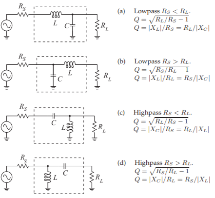
Figure \(\PageIndex{1}\): L matching networks consisting of one shunt reactive element and one series reactive element. (\(R_{S}\) is matched to \(R_{L}\).) \(X_{C}\) is the reactance of the capacitor \(C\), and \(X_{L}\) is the reactance of the inductor \(L\). Note that with a two-element matching network the \(Q\) and thus bandwidth of the match is fixed.

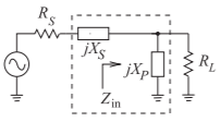
Figure \(\PageIndex{2}\): Two-element matching network topology for \(R_{S} < R_{L}\). \(X_{S}\) is the series reactance and \(X_{P}\) is the parallel reactance.

and the matching objective is \(Z_{\text{in}} = R_{S} − \jmath X_{S}\) so that

\[\label{eq:2}R_{s}=\frac{R_{L}X_{P}^{2}}{R_{L}^{2}+X_{P}^{2}}\quad\text{and}\quad X_{S}=\frac{-X_{P}R_{L}^{2}}{X_{P}^{2}+R_{L}^{2}} \]

From these

\[\label{eq:3}\frac{R_{S}}{R_{L}}=\frac{1}{(R_{L}/X_{P})^{2}+1}\quad\text{and}\quad -\frac{X_{S}}{R_{S}}=\frac{R_{L}}{X_{P}} \]

Introducing the quantities

\[\label{eq:4}Q_{S}=\text{ the }Q\text{ of the series leg }=|X_{S}/R_{S}| \]

\[\label{eq:5}Q_{P}=\text{ the }Q\text{ of the shunt leg }=|R_{L}/X_{P}| \]

leads to the final design equations for \(R_{S} < R_{L}\):

\[\label{eq:6}|Q_{S}|=|Q_{P}|=\sqrt{\frac{R_{L}}{R_{S}}-1} \]

The L matching network principle is that \(X_{P}\) and \(X_{S}\) will be either capacitive or inductive and they will have the opposite sign (i.e., the L matching network comprises one inductor and one capacitor). Also, once \(R_{S}\) and \(R_{L}\) are given, the \(Q\) of the network and thus bandwidth is defined; with the L network, the designer does not have a choice of circuit \(Q\).

Example \(\PageIndex{1}\): Matching Network Design

Design a circuit to match a \(100\:\Omega\) source to a \(1700\:\Omega\) load at \(900\text{ MHz}\). Assume that a DC voltage must also be transferred from the source to the load.

Solution

Here \(R_{S} < R_{L}\), and so the topology of Figure \(\PageIndex{3}\)(a) can be used and there are two versions, one with a series inductor and one with a series capacitor. The series inductor version (see Figure \(\PageIndex{3}\)(b)) is chosen as this enables DC bias to be applied. From Equations \(\eqref{eq:4}\)–\(\eqref{eq:6}\) the design equations are

\[\label{eq:7}|Q_{S}|=|Q_{P}|=\sqrt{\frac{1700}{100}-1}=\sqrt{16}=4,\quad\frac{X_{S}}{R_{S}}=4,\quad\text{and}\quad X_{S}=4\cdot 100=400 \]

This indicates that \(\omega L = 400\:\Omega\), and so the series element is

\[\label{eq:8}L=\frac{400}{2\pi\cdot 9\cdot 10^{8}}=70.7\text{ nH} \]

For the shunt element next to the load, \(|R_{L}/X_{C}| = 4\), and so

\[\label{eq:9}|X_{C}|=\frac{R_{L}}{4}=\frac{1700}{4}=425 \]

Thus \(1/\omega C = 425\) and

\[\label{eq:10}C=\frac{1}{2\pi\cdot 9\cdot 10^{8}\cdot 425}=0.416\text{ pF} \]

The final matching network design is shown in Figure \(\PageIndex{3}\)(c).

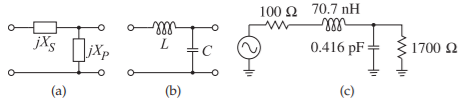
Figure \(\PageIndex{3}\): Matching network development for Example \(\PageIndex{1}\).

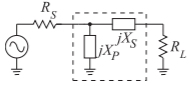
Figure \(\PageIndex{4}\): Two-element matching network topology for \(R_{S} > R_{L}\).

L Network Design for \(R_{S}>R_{L}\)

For \(R_{S} > R_{L}\), the topology shown in Figure \(\PageIndex{2}\) is used. The design equations for the L network for \(R_{S} > R_{L}\) are similarly derived and are

\[\label{eq:11}|Q_{S}|=|Q_{P}|=\sqrt{\frac{R_{S}}{R_{L}}-1} \]

\[\label{eq:12}-Q_{S}=Q_{P},\quad Q_{S}=\frac{X_{S}}{R_{L}},\quad\text{and}\quad Q_{P}=\frac{R_{S}}{X_{P}} \]

Example \(\PageIndex{2}\): Two-Element Matching Network

Design a passive two-element matching network that will achieve maximum power transfer from a source with an impedance of \(50\:\Omega\) to a load with an impedance of \(75\:\Omega\). Choose a matching network that will not allow DC to pass.

Solution

\(R_{L} > R_{S}\), so, from Figure \(\PageIndex{1}\), the appropriate matching network topology is

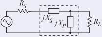
Figure \(\PageIndex{5}\)

This topology can be either high pass or low pass depending on the choice of \(X_{S}\) and \(X_{P}\). Design proceeds by finding the magnitudes of \(X_{S}\) and \(X_{P}\). In two-element matching the circuit \(Q\) is fixed. With \(R_{L} = 75\:\Omega\) and \(R_{S} = 50\:\Omega\).

The \(Q\) of the matching network is the same for the series and parallel elements:

\[|Q_{S}|=\frac{|X_{S}|}{R_{S}}=\sqrt{\frac{R_{L}}{R_{S}}-1}=0.7071\quad\text{and}\quad |Q_{P}|=\frac{R_{L}}{|X_{P}|}=|Q_{S}|=0.7071\nonumber \]

therefore \(|X_{S}| = R_{S}\cdot |Q_{S}| = 50\cdot 0.7071 = 35.35\:\Omega\). Also

\[|X_{P}|=R_{L}/|Q_{P}|=75/0.7071=106.1\:\Omega\nonumber \]

Specific element types can now be assigned to \(X_{S}\) and \(X_{P}\), and note that they must be of opposite type.

The lowpass matching network is

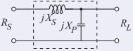
Figure \(\PageIndex{6}\)

\[X_{S}=+35.5\:\Omega,\quad X_{P}=-106.1\:\Omega\nonumber \]

The highpass matching network is

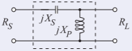
Figure \(\PageIndex{7}\)

\[X_{S}=-35.35\:\Omega ,\quad X_{P}=+106.1\:\Omega\nonumber \]

This highpass design satisfies the design criterion that DC is not passed, as DC is blocked by the series capacitor.

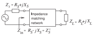
Figure \(\PageIndex{8}\): A matching network matching a complex load to a source with a complex Thevenin impedance.