
4: Persistent Data Storage
- Page ID
- 45737

Section 4:
Persistent Data Storage
Section Contents:
Learning Goals:
By the end of this section, you should be able to demonstrate:
- An understanding of basic database types
- How pieces of information can relate to each other
- The ability to normalize data into a structured query format
- The ability to create, populate, and interact with a MySQL database
- A basic understanding of the advanced capabilities of MySQL queries
Chapter 37
Database Types
While there are a number of databases available for use like MySQL, node.js, and Access, there is an additional list of the types of database structures each of these belong to. These types each represent a different organizational method of storing the information and denoting how elements within the data relate to each other. We will look at the three you are most likely to come across in the web development world, but this is still not an exhaustive representation of every approach available.
Flat File
Flat files are flat in that the entire database is stored in one file, usually separating data by one or more delimiters, or separating markers, that identify where elements and records start and end. If you have ever used Excel or another spreadsheet program, then you have already interacted with a flat file database. This structure is useful for smaller amounts of data, such are spreadsheets and personal collections of movies. Typically these are comma separated value files, .csv being a common extension. This refers to the fact that values in the file are separated by commas to identify where they start and end, with records marked by terminating characters like a new line, or by a different symbol like a colon or semi-colon.
The nature of all data being in one file makes the database easily portable, and somewhat human readable. However, information that would be repeated in the data would be written out fully in each record. Following our movie example, this could be the producer, studio, or actors. They have what we call a one-to-many relationship with other data in the database that cannot be tracked in this format.
Drawbacks to this format can affect your system in several ways. First, in our example, we would enter the studio name into each record for a movie made by that studio. If the person typing miss-typed an entry, it may not be found when users search the database, skewing search results through missing information. This often results in users creating new entries for a record that appears not to exist, causing duplication. Beyond search issues, every repetition is more space the database requires, especially when the value repeated is large. This was more of an issue when data was growing faster than storage capacity. Now, with exception to big data storage systems, the average user’s storage space on an entry level PC typically surpasses the user’s needs unless they are avid music or movie collectors. It is still important to consider when you are dealing with limited resources, such as mobile applications that are stored on smart phones that have memory limitations lower than that of desktops and servers.
Another issue with these files is the computational effort required to search the file, edit records, and insert new ones that are placed somewhere within the body of data as opposed to the start or end of the file.
Finally, flat files are not well suited for multiple, concurrent use by more than one party. Since all of the data is in one file, you are faced with two methods of interaction. The first approach is allowing anyone to access the file at the same time, usually by creating a local temporary copy on their system. While this allows multiple people the ability to use the file, if more than one party is allowed to make changes, we risk losing data. Say User 1 creates two new records while User 2 is editing one. If User 2 finished first and saves their changes, they are written back to the server. Then, User 1 sends their changes back, but their system is unaware of the changes made by User 2. When their changes are saved, User 2’s changes are lost as User 1 overwrites the file. This can be prevented by checking last modified timestamps before allowing data to be written, but the user “refreshing” may have conflicts between their edits and the edits from another user, when the same record is changed.
The alternate approach to allowing multiple users is to block multiple users from making changes by only allowing one of them to have the file open at a time. This is done by creating a file lock, a marker on the file the operating system would see, that would block other users from using an open file. This approach does not support concurrent access to the data, and again even allowing read rights to other users would not show them changes in progress that another user has not completed and submitted. Another downside to this approach is what is called a race condition—where multiple systems are trying to access a file, but are unable to do so because another has the file locked, stalling all of the programs trying to access the data.
This was a key element in a large scale blackout of 2003 that took place in the Northeast United States and part of Canada. A summer heat wave created significant strain on the power system as demand for air conditioning increased, resulting in the emergency shutdown of a power station. This station happened to be editing its health status in a shared file between itself and other stations, a method used to allow other stations to adjust their operational levels in response to their neighbors. The purpose of this file was to act as a protection method, warning of potential spikes or drops in power at individual facilities. When the plant using the file shutdown, the file remained locked as the computer using it did not have time to send a close file command. Unable to properly close the file with the systems down, other stations were unaware of the problem until power demand at their facilities rapidly increased. As these stations could not access the file due to the lock, a warning could not be passed along. Since the power stations were under increasing strain with each failure, a cascading affect occurred throughout the entire system. Admittedly an extreme result of file lock failure, it is a very real world example of the results of using the wrong tools when designing a system.
Structured Query/Relational Database
Structured query databases can be viewed similar to flat files in that the presentation of a section of data can be viewed as its own table, similar to a single spreadsheet. The difference is that instead of one large file, the data is broken up based on user needs and by grouping related data together into different tables. You could picture this as a multi-page spreadsheet, with each page containing different information. For example, continuing with our movie example, one table would contain everything about the studio—name, opening date, tax code, and so on. The next table would contain everything about the movies—name, release date, description, production cost etc. Finally we might have a table for actors, producers, and everyone else involved. This table would have their information like birthday, hometown, and more.
What we do not have yet is a way to link these elements together. There is also a lot of information we do not want to include, because we can determine it from something else. For example, we do not want to store the actors age, or we would have to update the table every year on their birthday. Since we already have their birth date, we can have the server do the math based on the current date and their birth date to determine how old they are each time it is asked.
To address relating an actor in our people table to a movie they were in from the movie table, as well as to the studio that made the movie in the studio table, we use a structured query. Structured query is a human readable (relatively) sentence style language that uses a fixed vocabulary to describe what data we want and how to manipulate it. Part of this comes from adding extra tables. Since one actor can be in many movies, and each movie can have many actors, we have a many-to-many relationship between them. Due to this, we create an extra table where each row represents a record of an actor and a movie they were in. Instead of putting their full names into this table, we put the row number that identifies their information from their respective tables. This gives us a long, skinny table that is all numbers, called an “all-reference table,” as it refers to other tables and does not contain any new information of its own. We will see this in action soon.
We can use our query language to ask the database to find all records in this skinny table where the movie ID matches the movie ID in the movie table, and also where the movie name is “Die Hard.” The query will come back with a list of rows from our skinny table that have that that value in the movie ID column. We can also match the actor IDs from a table that pairs actors with movies to records in the actor table in order to get their names. We could do this as two different steps or in one larger query. In using the query, we recreate what would have been one very long record in our flat file. The difference is we have done it with a smaller footprint, reduced mistyping errors, and only see exactly what we need to. We can also “lock” data in a query database at the record level, or a particular row in a database, when editing data, allowing other users access to the rest of the database.
While this style can be very fast and efficient in terms of storage size, interacting with the data through queries can be difficult as both one-to-many and many-to-many relationships are best represented through intermediary tables like we described above (one-to-one relationships are typically found within the same table, or as a value in one table directly referencing another table). In order to piece our records together, we need an understanding of the relationships between the data.
MySQL
Structured query language databases are a very popular data storage method in web development. While different approaches are emerging to address big data issues, the concepts you learn by studying structured query can help you organize data in any system.
MySQL, commonly pronounced as “my seequl” or “my s q l,” is a relational database structure that is an open source implementation of the structured query language. The relational element arises from the file structure, which in this case refers to the fact that data is separated into multiple files based on how the elements of the data relate to one another in order to create a more efficient storage pattern that takes up less space.
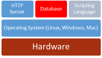
In a traditional LAMP, MySQL plays the role of our data server, where we will store information that we want to be able to manipulate based on user interaction. Contents are records, like all the items available in Amazon’s store. User searches and filters affect how much of the data is sent from the database to the web server, allowing the page to change at the user’s request.
History
MySQL began when developers Monty Widenius and David Axmark attempted to use the mSQL database system to interact with their own tables they had created using low-level routines in ISAM. Their testing did not reveal the speeds or flexibility they wanted, so they created their own similar API, and dubbed it MySQL after co-founder Monty’s daughter My.
After an internal release in 1995, MySQL was opened to the public with minor version updates spanning 3.19 to 3.23 from 1996 to 2000. Their next major version release, 4.0, arrived as beta in 2002 and reached production in 2003. Their next major release arrived as 5.0 in 2005 and included the addition of cursors, stored procedures, triggers, and views. These were all significant additions to the toolset.
In 2008, Sun Microsystems acquired what was then called MySQL AB with an agreement to continue development and release of the software as a free and open source item. When Sun was acquired by Oracle in 2010, MySQL was part of the package deal, under the same requirements. There have been some arguments over whether or not the spirit of the agreement between MySQL and Sun has been fully upheld by Oracle, including complaints from Widenius himself.
Structure
We organize data in MySQL by breaking it into different groups, called tables. Within these tables are rows and columns, in which each row is a record of data and each column identifies the nature of the information in that position. The intersection of a row and column is a cell, or one piece of information. Databases are collections of tables that represent a system. You can imagine a database server like a file cabinet. Each drawer represent a database in our server. Inside those drawers are folders that hold files. The folders are like our tables, each of which holds multiple records. In a file cabinet, our folders hold pieces of paper or records, just like the individual rows in a table. While this may seem confusing now, we will see it in action soon; this is the approach we will focus on for this section of the text.
NoSQL
NoSQL databases represent systems that maintain collections of information that do not specify relationships within or between each other. In reality, a more appropriate name would be NoRel or NoRelation as the focus is on allowing data to be more free form.
Most NoSQL system follow a key-value pairing system where each element of data is identified by a label. These labels are used as consistently as possible to establish common points of reference from file to file, but may not be present in each record. Records in these systems can be represented by individual files. In MongoDB, the file structure is a single XML formatted record in each file, or it can be ALL records as a single XML file. Searching for matches in a situation like this involves analyzing each record, or the whole file, for certain values.
These systems excel when high numbers of static records need to be stored. The more frequently data needs to be changed, the more you may find performance loss here. However, searching these static records can be significantly faster than relational systems, especially when the relational system is not properly normalized. This is actually an older approach to data storage that has been resurrected by modern technology’s ability to capitalize on its benefits, and there are dozens of solutions vying for market dominance in this sector. Unless you are constructing a system with big data considerations or high volumes of static records, relational systems are still the better starting place for most systems.
Learn more
Keywords, search terms: Database types, data structures, data storage
Node.js: http://nodejs.org/
The Acid Model: http://databases.about.com/od/specificproducts/a/acid.htm
Key-Value Stores, Marc Seeger: http://blog.marc-seeger.de/assets/papers/Ultra_Large_Sites_SS09-Seeger_Key_Value_Stores.pdf
Chapter 38
Data Relationships
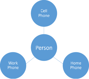
Before we begin to design our database, we need to understand the different relationships that can exist between two pieces of information. For this example, we will start with two imaginary tables. The first will be names, and the second will be phone numbers. If we first consider a person with a cell phone that has no other numbers they can be reached at, we see a one-to-one relationship—the phone number for that cell phone is the only one associated with that person, and that person is the only one you reach when you call that number.
 This does not cover all phone uses, though. Many of us still have phones at home or at work that are used by multiple people. In this case, the relationship between that phone and its users is one-to-many, as more than one person can be reached by using that phone number.
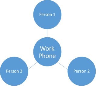
 In reality, both of these are probably true for most people. This means that one number can represent many people (calling a house or business) and one person can be reached via multiple phone numbers. In this case, we have a many-to-many relationship where multiple values of the same table can relate to multiple values of another table. In this example, of all numbers (work, home, or cell) are stored in the same table, there can be multiple values connected to either side of a given number.
 When we apply the theory of normalization to the database we are about to design, it is important to keep these relationships in mind as it indicates how we should structure our database. A one-to-one relationship can be resolved by keeping both pieces of information in the same table or by including a reference in either of the two tables to the other. For one-to-many relationships we need to keep the data in separate tables, and refer to the “one” item in our “many” table. Finally, for many-to-many relationships we do not have a good way to link directly between tables without violating normalization methods; instead we will create small connecting tables where each record represents a valid combination of the items from our two tables.
Primary, Foreign Keys
To find information in our database we need to be able to uniquely identify the record(s) we want to interact with. This can be done several ways. First, we can identify a piece of information from our table that makes each record unique, like a social security number identifies a US citizen. Sometimes, however, our record does not have one single piece of information that does this. Take a home address for example. To make an address unique, we need to take the street name, number, city, and zip code at a minimum. We can use this method to create a key that uses more than one column to identify a record, called a hybrid key.
Our last method is to let the database make a key for us, so every time we insert a record it receives a number unique for that table automatically. In this method, we let the database manage an auto-increment for that column. While it identifies a particular row, it does not contribute information that relates to the data it identifies. We will see examples of primary keys come into play as we normalize an example dataset, so for now you just need to keep the concept in mind.
Chapter 39
MySQL Data Types
The next few pages will likely be a little dry. Apologies now. However, whenever we create a table structure in MySQL we must identify the data type we intend to store in any given column, and depending on the type of data and other features we may want, this is just the beginning. Since one of our goals in the relational approach to database design is reducing overall size, it is also important to consider the best fit data type for what we want to store. Familiarizing yourself with the types available in MySQL will lend to your ability to design efficient table structures. The tables below are adopted from http://www.w3resource.com/mysql/mysql-data-types.php. They have been trimmed down in an attempt to not introduce an overwhelming amount of detail. You are encouraged to review the original version for more depth.
Integer Types
|
Type |
Length in Bytes |
Minimum Value(Signed/Unsigned) |
Maximum Value(Signed/Unsigned) |
|
TINYINT |
1 |
-128 to 0 |
127 to 255 |
|
SMALLINT |
2 |
-32768 to 0 |
32767 to 65535 |
|
MEDIUMINT |
3 |
-8388608 to 0 |
8388607 to 16777215 |
|
INT |
4 |
-2147483648 to 0 |
2147483647 to 4294967295 |
|
BIGINT |
8 |
-9223372036854775808 to 0 |
9223372036854775807 to 18446744073709551615 |
Floating-Point Types
|
Types |
Description |
|
FLOAT |
A precision from 0 to 23 results in a four-byte single-precision FLOAT column. |
|
DOUBLE |
A precision from 24 to 53 results in an eight-byte double-precision DOUBLE column. |
Fixed-Point Types
|
Types |
Description |
|
DECIMAL |
In the format DECIMAL(precision,scale). Maximum number of digits allowed are 65 before MySQL 5.03 and 64 after 5.03. |
|
NUMERIC |
Same as DECIMAL. |
Bit Value Types
|
Types |
Description |
|
BIT |
In the format b BIT(N), where N is an integer. |
Numeric type Attributes
|
Types |
Description |
|
TYPE(N) |
Where N is an integer and display width of the type is up to N digits. |
|
ZEROFILL |
The default padding of spaces is replaced with zeroes. So, for a column INT(3) ZEROFILL, 7 is displayed as 007. |
DATETIME, DATE, and TIMESTAMP Types
|
Types |
Description |
Display Format |
Range |
|
DATETIME |
Use when you need values containing both date and time information. |
YYYY-MM-DD HH:MM:SS |
‘1000-01-01 00:00:00’ to ‘9999-12-31 23:59:59’. |
|
DATE |
Use when you need only date information. |
YYYY-MM-DD |
‘1000-01-01’ to ‘9999-12-31’. |
|
TIMESTAMP |
Values are converted from the current time zone to UTC while storing, and converted back from UTC to the current time zone when retrieved. |
YYYY-MM-DD HH:MM:SS |
‘1970-01-01 00:00:01’ UTC to ‘2038-01-19 03:14:07’ UTC. |
String Types
|
Types |
Description |
|
CHAR |
Contains non-binary strings. Length is fixed as you declare while creating a table. |
|
VARCHAR |
Contains non-binary strings. Columns are variable-length strings. |
BINARY and VARBINARY Types
|
Types |
Description |
Range in bytes |
|
BINARY |
Contains binary strings. |
0 to 25. |
|
VARBINARY |
Contains binary strings. |
A value from 0 to 255 before MySQL 5.0.3, and 0 to 65,535 in 5.0.3 and later versions. |
BLOB and TEXT Types
|
Types |
Description |
Categories |
Range. |
|
BLOB |
Large binary object that containing a variable amount of data. Values are treated as binary strings. You do not need to specify length while creating a column. |
TINYBLOB |
Maximum length of 255 characters. |
|
MEDIUMBLOB |
Maximum length of 16777215 characters. |
||
|
LONGBLOB |
Maximum length of 4294967295 characters. |
||
|
TEXT |
Values are treated as character strings having a character set. |
TINYBLOB |
Maximum length of 255 characters. |
|
MEDIUMBLOB |
Maximum length of 16777215 characters. |
||
|
LONGBLOB |
Maximum length of 4294967295 characters. |
ENUM Types
A string object whose value is chosen from a list of values given at the time of table creation. For example:
- ENUM('small', 'medium', 'large')
SET Types
A string object having zero or more comma separated values (maximum 64). Values are chosen from a list of values given at the time of table creation.
Chapter 40
Normalization
Normalization is the process of structuring and refining the data we want to store in such a way that we eliminate repeated information and represent as much connection between records as possible. When a database meets particular rules or features of normalization, it is usually referred to as being in a particular normal form. The collection of rules progress from the least restrictive (first normal, or 1NF) through the most restrictive (fifth normal, or 5NF) and beyond. Databases can still be useful and efficient at any level depending on their use, and anything beyond third normal form is more of a rarity in real world practice.
Bear in mind, that normalization is a theory on data organization, not law. Your database can operate just fine without adhering to the following steps, but following the process of normalizing will make your life easier and improve the efficiency of your website. Not every set of circumstances will require all of these rules to be followed. This is especially true if they will make accessing your data more difficult for your particular application. These rules are designed to help you eliminate repeated data, are able to keep your overall database size as small as possible, and create integrity in your records.
Zero Normal Form
To begin, we need something to normalize. Through this section we will create a database to keep track of a music collection. First, we need a list of what we want to track. We will follow what is generally useful for a collection of music, like albums, artists, and songs. These categories give us a list of things we want to store, so let us come up with what a full record might contain:
|
Band Name |
Album Title |
Song Title |
Song length |
Producer Name |
|
Release Year |
Artist hometown |
Concert Venue |
Concert Date |
Artist Name |
To get a visual of what this table might look like, let us take a look at some sample data with many of these fields:
|
SONG TITLE |
ARTIST |
GENRE |
SUB-GENRE |
YEAR |
|
Shannon |
Henry Gross |
Rock |
Light Rock |
1976 |
|
Lover’s Will |
Bonnie Raitt |
Rock |
Light Rock |
1998 |
|
I Don’t Wanna Live Without Your Love |
Chaptercago |
Rock |
Light Rock |
1988 |
|
Heart Attack |
Olivia Newton-John |
Pop |
Adult Contemporary |
1982 |
|
In A Dream |
Badlands |
Rock |
Hard Rock |
1991 |
|
With A Little Luck |
Paul McCartney |
Rock |
Classic Rock |
1978 |
|
It’s A Miracle |
Barry Manilow |
Pop |
Adult Contemporary |
1975 |
|
It’s Only Love |
Bryan Adams / Tina Turner |
Pop |
Adult Contemporary |
1984 |
|
Jazzman |
Carole King |
Pop |
Adult Contemporary |
1974 |
|
Jesse |
Carly Simon |
Pop |
Adult Contemporary |
1980 |
|
Just Like Jesse James |
Chapterr |
Pop |
Adult Contemporary |
1989 |
|
Little Miss Cannot Be Wrong |
Spin Doctors |
Pop |
Adult Contemporary |
1992 |
|
Lost In Love |
Air Supply |
Pop |
Adult Contemporary |
1980 |
|
Good Times |
Sam Cooke |
Hip-Hop |
Soul |
1964 |
|
Make It With You |
Bread |
Pop |
Adult Contemporary |
1970 |
|
Mandy |
Barry Manilow |
Pop |
Adult Contemporary |
1974 |
|
Miss Chaptertelaine |
K.D. Lang |
Pop |
Adult Contemporary |
1992 |
|
Never Gonna Fall In Love Again |
Eric Carmen |
Pop |
Adult Contemporary |
1976 |
|
People Get Ready |
Rod Stewart |
Pop |
Adult Contemporary |
1985 |
|
Try Honesty (Radio Version) |
Billy Talent |
Rock |
Modern Rock |
2007 |
|
Silver Threads And Golden Needles |
Linda Ronstadt |
Pop |
Adult Contemporary |
1974 |
|
So Far Away |
Carole King |
Pop |
Adult Contemporary |
1971 |
|
Fat Lip |
Sum 41 |
Rock |
Modern Rock |
2001 |
|
Thank You For Being a Friend |
Andrew Gold |
Pop |
Adult Contemporary |
1978 |
As an example of non-normalized or “zero normal form” data, you can look to the data above where you see long, repeated fields. While this table is easy to read without a query or software, it quickly becomes unmanageable even in its readable format as 25 records turns into just a few hundred.
Let us take a summary look at our forms that will help us tackle this problem:
First Normal Form
- Create separate tables for related information
- Eliminate duplicated columns within tables
- Create primary keys for each table
Second Normal Form
- Meet first normal form
- Move data that will repeat often into a reference table
- Connect reference tables with foreign keys
Third Normal Form
- Meet second normal form
- Eliminate columns that do not relate to their primary key
Fourth Normal Form
- Meet third normal form
- Has no multi-valued dependencies
When working with an existing data set like our example above, you can quickly move through normalization once you are familiar with the rules. By adjusting our table(s) until they meet each set of rules, our data becomes normalized. Since we are learning, we will formulate our database from scratch.
Additional notes
As we draw up our design, each bolded word represents a table, and the names underneath represent our columns. We can simulate a record, or row, in our database by writing out sample values for each thing in our list.
First Normal Form
To get started, we will go through our draft list piece by piece. “Band Name” refers to the official name of the group or artist we are talking about. A good question to ask is does the column sounds like a concept, object, or idea that represents something, or would have properties, in our database. The concept of a band for us is important, and it will have properties made up of other columns we plan to have, like songs and albums. Since we can see this is a concept, it is a good candidate for a table, so we will start by creating a table for our bands. Just like we studied in the PHP section, it is good practice to keep a set of conventions when naming elements. With databases, it can be helpful to treat your tables as the plural form of what its rows will contain. In this case, we will name our table Bands. Under this name, we will list “Band Name” to the list of information in that table. A key element to think about every time we consider adding a field to a table is to make sure it represents only one piece of information. A band name meets our criteria of being only one piece of information, so we are on track.
Now our design notes might look more like this:
|
Band Name |
Album Title |
Song Titles |
Song length |
Producer Name |
|
Release Year |
Artist hometown |
Concert Venue |
Concert Date |
Artist Names |
|
Bands Band Name |
|
|
Our next element, Album Title, seems like it would relate to a band. At first, we might be tempted to put it in the band table because the album record we add belongs to the band. However, when we consider our data relationships, it becomes clear that we have a one to many situation; one band will (one-hit wonders aside) release more than one album. Since we always program to meet our highest possible level of relationship, the one-hit-wonders will exist perfectly fine even with only one album in our database. If you recall, we address one to many relationships by placing the two sides in separate tables and identifying in the “many” table which “one” the record is paired with. To do this, we will make an albums table just like we did for bands, and add a placeholder in our note to refer to the band table:
|
Band Name |
Album Title |
Song Titles |
Song length |
Producer Name |
|
Release Year |
Artist hometown |
Concert Venue |
Concert Date |
Artist Names |
|
Bands Band Name |
Albums Album Name |
|
Now we are on to “Song Titles.” The songs are organized into albums, so we will add it in.
Albums
Album Name
Song Titles
Apply our tests and see if this works. Does this field represent one piece of information? Titles is plural as we have it written, but we cannot put more than one piece of information in a single cell. We will need to break that up into individual titles to resolve. To make that change in this table though, we would have to create a column for each track. In order to do that, we would need to know ahead of time the max number of tracks any album we enter will have. This is not only impractical, but violates our first normal form of not repeating columns. Through this we can see that we again have a one to many relationship on our hands as one album will have multiple tracks. To resolve this, once again we will break our multiple field out to its own table, where we can create a link back to our album table:
|
Band Name |
Album Title |
Song Titles |
Song length |
Producer Name |
|
Release Year |
Artist hometown |
Concert Venue |
Concert Date |
Artist Names |
|
Bands Band Name |
Albums Album Name |
Songs Song Title |
We can already see a thread weaving its way through our tables. Even though these fields are no longer all in one record together, you can see how we can trace our way through by looking for the band we want in the albums table, and when we know the albums, we can find all the tracks the band has published. To continue with our design we will move to song length. This field sounds fitting in our songs table, and is only one piece of information, so we are off to a good start! We can also see that we would only have one song length per record as each record here is a song, so we comply with column count, too. We can put it there for now, and will see if it meets the rest of our tests as we move on.
|
Band Name |
Album Title |
Song Titles |
Song length |
Producer Name |
|
Release Year |
Artist hometown |
Concert Venue |
Concert Date |
Artist Names |
|
Bands Band Name |
Albums Album Name |
Songs Song Title |
Now that we have an idea of first normal form, we will get the rest of our initial columns out of the way:
|
Band Name |
Album Title |
Song Titles |
Song length |
Producer Name |
|
Release Year |
Artist hometown |
Concert Venue |
Concert Date |
Artist Names |
|
Bands Band Name |
Albums Album Name |
Songs Song Title |
|
Labels Producer Name |
Artists Artist Name |
Concerts Venue |
Now that we have exhausted our initial list, we will consider the last element of 1NF, which is primary keys for each table. Many of our tables are not presenting us with good candidates, as band names, venues, albums, tracks, and even artists could share the same names as time goes on. To make things consistent, we will create auto incrementing IDs for each table. To follow best practices, we will use the singular version of the noun with ID after it to denote our primary keys. This identifies the row as a singular version of the concept our table name is a plural of:
|
Bands bandID |
Albums albumID |
Songs songID |
|
Labels producerID |
Artists artistID |
Concerts venueID |
Second Normal Form
We have now reached first normal form. Now I must admit, I have been a bit sneaky. By introducing data relationships, and showing you how to apply the relationship when considering where to put columns, we have already addressed part of second normal form, so, technically, we are already beyond first normal form. The first piece of second normal form is creating tables anywhere where a value of a cell could apply to multiple records of that table. When we moved song title out of albums, we were fulfilling this requirement. Looking over our tables again, we can see that, as we have things now, this has been met.
The other element of second normal form is that connections between tables should be facilitated by foreign keys. We have already started that process by earmarking a couple tables with notes where we knew we needed connections. Now that we have our primary keys, we have the unique values we will need to use. For this pass, we will look at how our tables relate to each other and see if we need connections. This is another step where remembering how to solve our data relationships will be important. To start with the tables we earmarked, we will look at “Albums.” Our reference calls for connecting it to “Bands,” so we will add a foreign key in “Albums” that points to “Bands.” To make things easy on us, we can use the same name in both tables so we know what it is for.
|
Bands bandID |
Albums albumID |
Songs songID |
|
Labels producerID |
Artists artistID |
Concerts venueID |
We can do the same with our “Songs” table as well to reference our “Albums” table. Looking at our “Labels” table, it could be argued that since a band belongs to a label that we should connect them. However, the relationship between a band and a label can change over time as contracts come and go, which would give us a many-to-many relationship. Another place we can associate this information is in the album. Once an album is published, the label that produced it will not change, and multiple labels do not publish the same album. To resolve these, we need album in two places. First, we need a many-to-many relationship table for labels and bands, and a one-to-many link between albums and labels. We already know how to link on-to-many, so we will add a foreign key to producerID in or albums table. Then we will add a table that has an incrementing auto ID, a foreign key to labels, and foreign key to albums, and a timestamp:
|
Bands bandID |
Albums albumID |
Songs songID |
|
|
Labels producerID |
Artists artistID |
Concerts venueID |
Bands2Labels id |
By adding the timestamp column in our many-to-many table, we can sort by the date the records were added, assuming they were added chronologically. This means the newest record would represent who the band is signed with now, and we can look at all the records with a particular band to see who a band has worked with, and we can look at all the records for a label to see who they have signed.
If we wanted to round out this information more, we could add start and end timestamps that represent contracts with the label. With the additional of these fields we could create even more timelines.
Continuing on, we have our “Artists” table. We know performers can be solo or in groups, and can belong to different bands over time, so we have another many-to-many relationship. You will notice the name given to the table bridging our bands and labels relationship is labelled Bands2Labels. This of course is only one possible name we could use, but is an example of how to clearly identify the purpose of the table, as we are linking “bands to labels.” Our last table to look at is “Concerts.” We need a way to associate a particular concert with the band that performed. Since each row of this table is a particular concert we will add a foreign key in.
We now have foreign keys to link our tables together where needed, and do not have a situation where multiple records in a table would contain the same values. We have now reached second normal form.
Third Normal Form
Our next normal form requires that all of the fields in a table relate to the key (or are a key), or in other words the concept of that table. In our smaller tables this is immediately apparent to us—a band name relates directly to a band, and a producer name relates directly to a label. It can be remembered in a popular rewording to the well-known court room oath that references Edgar Codd, who created the concept of third normal form. My favorite variation is the following: “All columns in the table must relate to the key, the whole key, and nothing but the key, so help me Codd”(source unknown).
To see third normal form in action we will review our current design. We already considered bands and labels while describing this form, so we will mark them green as OK.
|
Bands bandID |
Albums albumID |
Songs songID |
|
|
Labels producerID |
Artists artistID |
Concerts venueID |
Bands2Labels id |
When we review “Albums” and “Songs” we only have a couple fields to consider from each table as the rest are primary and foreign keys. Album names and release years both refer to albums, and the same holds true for song titles and length in the songs table. Bands2Lables is also easy to review as all of the elements are keys—it is an all-reference table.
|
Bands bandID |
Albums albumID |
Songs songID |
|
|
Labels producerID |
Artists artistID |
Concerts venueID |
Bands2Labels id |
Next, consider the “Artists” table. Artist name, obviously, fits with artist. What about hometown? Certainly they relate—a person usually identifies one location as home—but the actual information that would reside in the cell (likely a city) does not just relate to an artist. Looking at our concert table for example, a venue would have a physical location in which it resides as well. This tells us that hometown needs to be moved somewhere else. Since we do not have a place in our database that speaks specifically to locations, we will have to add one. When we do this, we should also consider that in reality the hometown city name by itself is not sufficiently unique without a state and zip code reference as well, and we will need to change our existing hometown column to reference the new table:
|
Bands bandID |
Albums albumID |
Songs songID |
||
|
Labels producerID |
Locations locID |
Artists artistID |
Concerts venueID |
Bands2Labels id |
Almost there! When we consider the “Concerts” table, at first glance we appear to be in third normal form (because we are). While we are here though, we need to keep in mind that in each pass of normalization we need to consider the database as a whole and all of the other forms of normalization as we keep tweaking our tables. Here, while venue makes sense as a column, using venue as the primary key seems confusing, as we are identifying a particular concert, not a particular place. When we consider this, it may also become apparent that just knowing the name of a venue may not be enough to uniquely identify it either. Since we have created a location table, we can take advantage of it here as well:
|
Bands bandID |
Albums albumID |
Songs songID |
||
|
Labels producerID |
Locations locID city state zip |
Artists artistID |
Concerts concertID locID |
Bands2Labels id |
Have we satisfied all forms? Well, not quite yet. We have adjusted our concerts table to better meet third normal form, but is it fully compliant or did we miss something? Imagine this table populated and you will notice that the venue field—the name of our location—would be repeated each time the venue was used. This violates second normal form. To solve this, we know we need to split the data out to its own table, so we need to see if anything else should go with it. The location ID we just created relates to the venue, not the event, so that should go too. The date is correct where it is, as it identifies a particular piece of information about the concert. Does this cover everything? We do not seem to have a means to identify who actually performed the concert at that venue on that date, do we? This is a key piece of information about a concert, and any given concert usually involves more than one performer. Not only do we need to add the field but we need to remember our data relationships and see that this is a many-to-many between artists and concerts. Multiple artists can perform at the same event, and with any luck a given artist will perform more than one concert. We can address all of these changes by creating a Venues table, a many-to-many reference table for concerts and performers, and adjusting our concerts table to meet these changes. Try writing it out yourself before looking at the next table!
|
Bands bandID |
Albums albumID |
Songs songID |
Concerts2Artists Id |
||
|
Labels producerID |
Locations locID |
Artists artistID |
Venues venueID |
Concerts concertID Date |
Bands2Labels id |
Now, all of the tables we had at the beginning of third normal form are complete. We need to review the three we created to make sure they, too, meet all three forms. In this example, they do.
Now that we have reached third normal form we can see how normalization helps us out. We could have a list of 2000 concerts in our system, and each of those records would just be numerical references to one record for each artist and concert. In doing this, we do not of repeat all of those details in every record.
Fourth Normal Form
While most systems (and most tutorials) usually stop at third normal form, we are going to explore a bit further. Fourth normal form is meant to address the fact that independent records should not be repeated in the same table. We began running into this when we looked for problems in complying with second normal form as we began to consider the data relationships between our fields. At the time, not only did we split out tables where we found one-to-many relationships, we also split out all-reference tables to account for the many-to-many relationships we found. This was easy to do at the time as we were focused on looking for those relationship types. That also means, however, that we have already met fourth normal form, by preventing many-to-many records from creating repeated values within our tables.
To keep fourth normal compliance in other systems, you will need to be mindful of places where user-submitted data could be repeated. For example, you may allow users to add links to their favorite sites. Certainly at some point more than one user will have entered the same value, and this would end up repeated in the table. To prevent this, you would store all links in a table and create a many-to-many reference with your user records. Each time a link is saved, you would check your links table for a match, update records if it exists, or add it to the table if it has never been used.
This process can be helpful when you expect very high volumes of records and/or need to be very mindful of the size, or footprint, of your database (for example, running the system on a smartphone).
Before we move on, we will make one more pass to clean up our design. Since we started with words as concepts, but want to honor best practices when we create our database, we will revise all of our tables to follow a consistent capitalization and pluralization pattern:
|
Bands bandID |
Albums albumID |
Songs songID |
Concerts2Artists id |
||
|
Labels producerID |
Locations locID |
Artists artistID |
Venues venueID |
Concerts concertID |
Bands2Labels id |
Congratulations, you now have a normalized database! Flip back to look at our original design, and you will see a number of trends. First, the process was a bit extensive, and turned into far more tables than you likely expected. However, it also helped us identify more pieces of information that we thought we would want, and helped us isolate the information into single pieces (like splitting location in city, state, zip) which allows us to search by any one of those items.
Learn more
Keywords, search terms: Normalization, boyce-cobb normal form
MySQL’s Guide: http://ftp.nchu.edu.tw/MySQL/tech-resources/articles/intro-to-normalization.html
High Performance MySQL: http://my.safaribooksonline.com/book/-/9781449332471
Chapter 41
MySQL CRUD Actions
There are four basic actions that cover how we interact with the data and structures in our database. We can either create new data, read existing data, update something already in place, or delete it. These four actions are collectively referred to as CRUD, for Create Read Update and Delete, and represent the basic concepts behind data interaction. In MySQL, we will address these concepts through a collection of commands.
Opening SQL
From a Browser
If you are using an installation of WAMP, you will have access to PhpMyAdmin from your browser. This program includes a SQL tab where you can input commands to your server as well as use a graphic interface to interact with your databases. Typically you can get there by going to http://locahost/phpmyadmin or http://127.0.0.1/phpmyadmin (do not forget to add the port number if you changed yours from :80). Your credentials will be the same as described in the next section, and you will find a SQL tab that allows you to enter commands to follow along with our examples.
From a Command Prompt
Each MySQL installer includes a client access program to interact with your server. Due to the variety of operating systems and versions of MySQL, definitive directions for accessing your client program cannot be provided here, but can be found by searching online with the details of your particular system. In general, your programs list may contain a MySQL folder with a link to launch the client, or you can access it by using your system’s terminal window. Once you have a terminal window open, you can log into MySQL by typing:
- mysql –u root –p
This instructs your computer to start MySQL using the username (represented by –u) of root and asking it to prompt you for a password, represented by –p. Once you press enter, you will be prompted to enter the password. By default, MySQL uses root as the username. Your password could be root, password, or an empty password (type nothing at all) depending on your version. If you changed these values when you installed, use what you provided in place of this example.
Once logged in to your database, you can begin to take a look around to see what your server already contains. To see what is currently in your server, you can enter a simple command to ask for that list. In MySQL we need to end our statements with semi-colons just as we do with PHP. Our commands and interactions are structured to be sentence-like, which makes queries easier to understand. Let us take a look at what we have available:
- Show databases;
In a new installation of MySQL, you should see a list similar to the following:
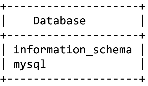
- 2 rows in set (0.00 sec)
Now that we have designed our database, it is time to describe it to the server, and get some data into it, so we have a fully functioning system. First we need to get into MySQL:
- create database music;
After pressing enter you should see a response from the server that gives either a completed message or an error message, along with other information such as the amount of time it took to complete the instruction. If you receive an error that the database already exists, you can use a different name. If something happened and you are starting over, or know you can get rid of the existing database, you can get rid of it and all its data by typing:
- drop database music;
Keep in mind this command deletes everything—the database and all tables and data stored in it. There is no “undo” option or garbage bin to recover from, so if you do not have a backup you will not be able to recover from this action. Once you have a database created, tell the server that is the one you want to interact with by typing:
- use music;
You will notice we consistently use semi-colons after each instruction. Just like in PHP, this is how the server can tell where one instruction ends and the next begins.
Create
The first step in building our database is to create the tables from our design. Before we do so, we need to create the database we want to put those tables in. Be sure you have a music database created as we saw above. We will keep using the database we just designed. The create command for a table involves specifying that we mean to create a table (as opposed to a database), defining our table name, and then in parenthesis defining each column. This done with a comma separated collection of values that includes the name, type, null option, and other features of the column. Here we will look at the command necessary to create our first table:
|
Bands bandID |
Albums albumID |
Songs songID |
Concerts2Artists id |
||
|
Labels producerID |
Locations locID |
Artists artistID |
Venues venueID |
Concerts concertID date |
Bands2Labels id |
- Create table bands (bandID int not null auto_increment primary key,
- bandName varchar (40) not null
- );
You will notice a few things about this statement. First, we only use commas to separate the entire definition of one column from another as opposed to separating each piece of information about a column. If you are using a command line interface, you can also use the enter key to format your statement as we did above, with one column on each line. This is due to the fact that the statement will not execute until the semicolon is present.
After we identified our first column as bandID, we identified it as an integer, referencing the data types we looked at earlier. We also stated that this column cannot be null, meaning it must have a value. We can apply this on any column that must be present in our table for a record to be considered useable. In this case, we want bandID to be entered for us by the database. Adding the auto_increment attribute will tell the database to assign each new record a value (we can also control the starting value if we ever wanted to start at something other than 1). Finally, we label this column as the primary key of our table, place a comma at the end of our definition, and move to the next column.
When we add our bandName to the table definition we needed to define far less. This time, we went with varchar (variable character) which means we expect the content to be text, but not necessarily long text like sentences or paragraphs. When we use varchar, we have to tell MySQL what the maximum number of characters is allowed in the field, so it knows how much space to reserve for each record. In this example, we have decided that our longest band name would be at most 40 characters. To complete this column we again specify that it cannot be null. In our example, it is the only field in the table outside of the id anyway. If we wanted to allow a null value, we could include the word null in place of not null, or just drop that piece altogether (MySQL will assume null is valid unless told otherwise).
After we execute this statement, we can use the command “show tables” to see what is in our database:
- mysql> show tables;
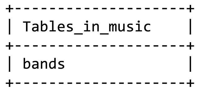
- 1 row in set (0.00 sec)
To make sure everything was created as we intended, we can look more closely at the structure of the table we created with the command “show columns from”:
- mysql> show columns from bands;
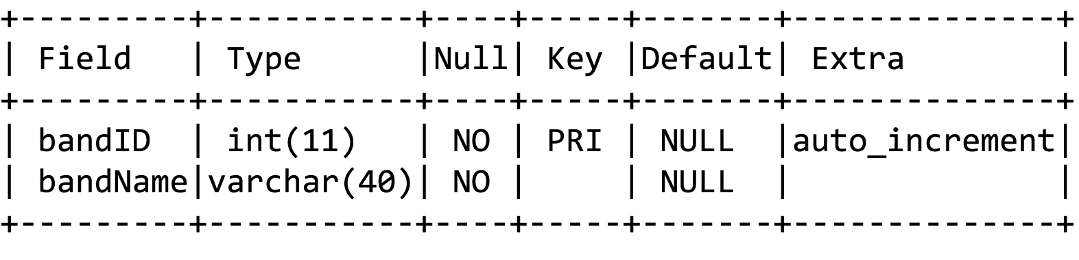
- 2 rows in set (0.02 sec)
Here we can see the structure of what we just created. Neither field can be null, bandID is our primary key, will auto increment, and neither field has a default value. If we want to assign a default value, we would include the word default followed by the value in quotation marks when defining our column.
We will create one more table here as a second example, and then you can continue creating the rest on your own in order to practice. Now we should create the Albums table so we can see a data field in use, which will cover all of the data types we will need in this database. Keep in mind that when we create tables with foreign keys in our example here, we are not going to define them as such at the database layer like we did when we defined our primary key. This is an available feature however, and allows MySQL to help us maintain data integrity by giving us an error if we try to insert a record where a foreign key value does not exist. As an example, if we tried to create a concert record but our reference to artist #5 did not exist in the artist table, MySQL would return an error instead of allowing the record to be created. You would have to create artist #5 first, then go back and try your previous statement again. Since this complicates the order of table creation and data insertion, we will ignore if for now until you are more comfortable, but know it is available and useful for production systems.
- Create table albums( albumID int not null auto_increment primary key,
- albumName varchar(70) not null,
- releaseDate date,
- bandID int not null,
- producerID int
- );
Once we have created all of our tables, we will need to put some data in them so we have something to interact with. To do this, we use the insert command. Using insert involves specifying the table we want to interact with, passing the list of fields we intend to fill, and then passing the values for those fields. The fields, as well as each set (or record) of values are contained in a comma separated list enclosed in parenthesis. Multiple records can be added at once, assuming each record is using the same set of fields, by adding another set of data in parenthesis. We can see this in action by creating our first band:
- Insert into bands(bandName) values ("The Who");
If we want to pass more than one record, we just keep tagging on more sets:
- Insert into bands(bandName) values ("Moxy Fruvous"), ("The Doors"), ("Maroon 5");
Take note of the fact that we do not specify the bandID for these records. Before we can insert albums though, we need to know what each band’s ID actually is. We will take a quick preview of the Read actions by using the following command to get that information:
- Select * from bands;
This command should give you something like the following:
- mysql> Select * from bands;

- 4 rows in set (0.00 sec)
Now we can use these values to try an insert that uses multiple columns. Keep in mind that if you try to insert a record without including a required field you will still get an error even if you do not include it in the fields you wish to pass! We also need to format our date to meet what MySQL expect, or need to use a MySQL function to convert it to something valid. Here we will format it ourselves. The default format is YYYY-MM-DD meaning four digit year, two digit month, two digit day, all separated by dashes:
- Insert into albums(albumName, bandID, releaseDate) values ("Tommy", 1, "1969-05-23"), ("Bargainville", 2, "1993-07-20"), ("Full Circle", 3, "1972-07-17");
As you can see in this example, complex values like strings and dates need to be wrapped in quotation marks so MySQL knows where they start and end, but we can leave basics like integers as they are.
Read
Now that we have some sample data, we will look at some basic techniques to see what we have. This is done with use of the select command, which comes with an assortment of filters and qualifiers. This is where the power of an SQL database comes into play as we manipulate, combine, and alter the information into what we want to see. We already saw one example of this when we needed to reference our bands table. The star that we used in “select * from bands” is a reserved character in MySQL that represents “all.” What we effectively asked was “select everything in the bands table.” We can drop the fields we do not want to see by specifying only the ones we want. For example, we can take a look at our albums table, but since we did not include producers yet and do not care about the record ID, we will just ask for certain columns:
- Select albumName, bandID, releaseDate from albums;

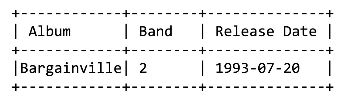
This gives us a more readable response. We will learn how to get the actual bandName soon, for now we will focus on how to change what we ask for. If we wanted to make this output more end-user friendly, we probably do not want to use the field names stored in the database. We can mask those by giving them an alias. We will also add some sorting in this example by applying the ascending sort (asc) in an order by clause to the album name (descending would be desc):
- Select albumName as "Album", bandID as "Band", releaseDate as "Release Date" from albums order by albumName asc;

We can also search for partial matches of text. Here we will use the “like” and “where” reserved words to further specify exactly what we want to see. You are probably noticing that most of our statements so far have been relatively human readable, meaning you can understand what is being done, just by reading the code. This is an intentional approach in structured query design as it makes it easier to design and debug more complex queries. Commas are used where more than one item is specified, however there is no comma after the last item in a list. You can see this where we do not include a comma after release date before moving on to specify the table we want in our “from” clause. You will also notice the use of % in the next example. This is another reserved character in MySQL, which represents a wild card, meaning anything found in that position is valid. In our example we will be searching for the word bargain, and because it is flanked on both sides by a % it will be considered a match anywhere in a string. If we only want things that start with bargain, we would only use the % after it.
- Select albumName as "Album", bandID as "Band", releaseDate as "Release Date" from albums where albumName like "%bargain%" order by albumName asc;
You may have noticed that our search string had bargain lowercase, but MySQL still returned Bargainville even though it is capitalized. This case-insensitive search is the default on MySQL, but you can specify particular form of upper or lowercase if you want. If we want to match only a specific string, we can use = in place of like and %. In fact, we can use many of the operators we are already accustomed to when numbers are involved, such as greater than and less than.
We should add a few more records to see some more of the options we have at our disposal when selecting data:
- Insert into albums(albumName, bandID, releaseDate) values ("Strange Days", 3, "1967-10-16"), ("Live Noise", 2, "1998-05-19");
Now we have a couple bands with more than one album. We can actually infer more data than we are storing in the database by using MySQL functions to manipulate the data and results in real time. Try using the count() function to find out how many albums we have for each artist. We need to specify what we want to count (in this case, records, so we can just use *) and what piece of the record we want to group to be counted, in this case the bandID:
- Select bandID, count(*) as "Albums" from albums group by bandID;
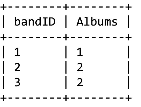
We are not actually storing the total number of albums in any of our tables—MySQL is tracking the total number of each time a bandID occurs from the group by statement.
Maybe we want to answer a question, like which album was released most recently? If this were an excel document, we would just sort the table by the release date and look at the first record. We can do the same thing in MySQL by adding a limit in the number of records we want back. While we could certainly take the whole table result and read just the first row, when your data set gets larger you do not want to send your user more data than they want or need, because it is wasteful of resources and can degrade the user experience (as well as increase demands on your server).
- Select * from albums order by releaseDate desc limit 1;
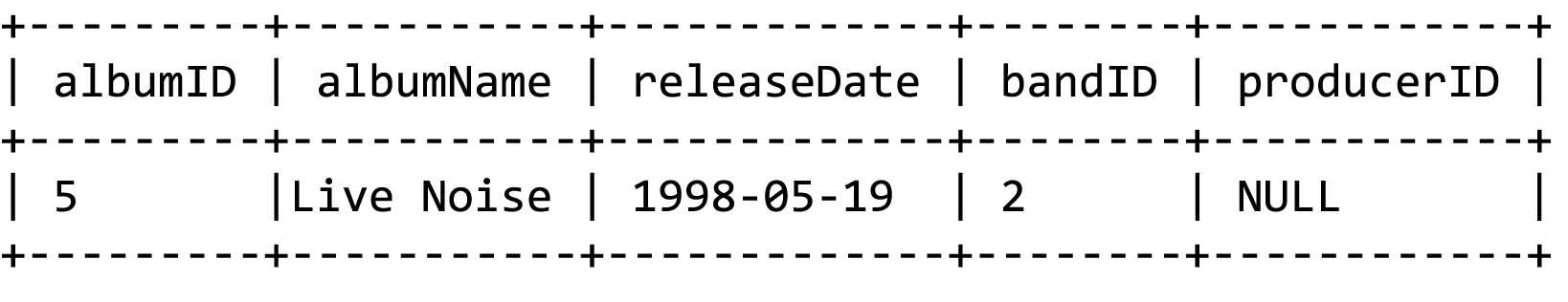
As a final example of some of the vocabulary available to us, we can also use the words “and” and “or” to add additional conditions to a statement:
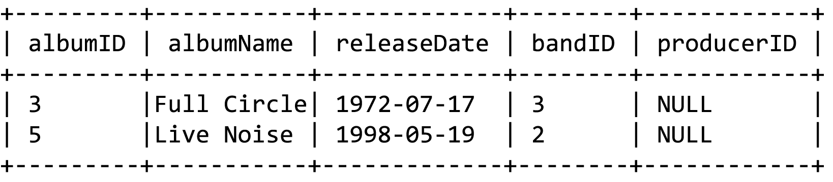
- Select * from albums where albumName like "%noise%" or albumName like "%circle%";
Keep in mind we are just touching the surface of the power of MySQL here. There are more reserved words, actions, abilities, and a whole library of functions that allow you to do even more.
Update
Now that we have practiced a bit of reading, we will try the next CRUD method, updating. Maybe instead of leaving the producerID as null we decide that we want it to say unknown by default. Since the producerID field is a foreign key reference, we cannot just change the value to text (we could use the Alter command to change the table structure, but this is out of our scope and would break our normalization). Since we only want to change the records where we do not have a producerID (even though in our case it is all of them) we need to specify that we want to change the column where the field is null. For update, we need to specify the table, define what we want our field set to, and the condition(s) required for the update to occur. Before we do this, we need a record in our Labels table where the producer name is “unknown.” We will pretend it is our first record:
- Update albums set producerID=1 where producerID is null;
Now, all of our records will show “unknown” when we begin to join tables. This keeps us from having to create extra code in our site to adjust output when the field would otherwise be empty.
If you want to change your values back, you can reset the whole column by setting the value without adding a where clause:
- Update albums set producerID=null;
Delete
The final CRUD method, delete, is as final as it sounds. Use with extreme caution! There is no “undelete” or “undo” function at our disposal. The vast majority of the time, it is best practice to never allow your users to delete records. Instead, add flags to your records that will hide the data from ever appearing again, by adding a Boolean “disabled” column to each table or creating a disabled table that tracks records that should not be shown (just a couple examples, there are even more ways to do this!).
As partial protection to the fast-fingered typists, MySQL splits delete functions out to two keywords, delete and drop. Delete is reserved for row-level actions, while drop is reserved for table and database level actions. Dropping a table or database is as simple as typing “drop table [your table name here]” or “drop database [your database name here].” There will be no “are you sure” prompt either. If the value exists, it will be removed. In terms of deleting rows, the same holds true. We define the table we want to interact with, and the conditions that identify rows we want deleted. We will remove any albums with “live” in their name as an example:
- Delete from albums where albumName like "%live%";
You should receive a response that says one row was affected, and if you review your whole table you will see that the Live Noise album is now gone.
Learn more
Keywords, search terms: CRUD, structure query languages, SQL, MySQL
MySQL Functions List: http://dev.mysql.com/doc/refman/5.0/en/func-op-summary-ref.html
Beginner Tutorials: http://beginner-sql-tutorial.com/sql.htm
Chapter 42
Advanced Queries
To use relational databases to their fullest extent, we need to be able to connect our tables using our foreign keys in order to extract our full records. This is done by combining statements and joining tables together.
Joining
We can join tables a number of ways. The primary portion of the join is specified in our where clause, which is where we will specify which fields between the two tables are to be connected. The simplest join will return only the records from the two tables where the value is found in both tables. We will begin by getting all the values from our albums and bands tables so we can finally see the band name in our results:
- Select * from bands, albums where album.bandID=bands.bandID;
You now probably have a messy looking table, but all our fields are there. Now, we can cut it back to just a simple list:
- Select bands.bandName as "Band", albums.albumName as "Album", releaseDate as "Released" from bands, albums where albums.bandID=bands.bandID;

You will notice we started to append the table name and a period before each field name. This helps clarify which field we are referring to when the same field name is used in more than one table. As a best practice, you may wish to always use this dot notation when selecting fields as it will help “future-proof” your queries if you expand or alter your database in the future, even if the field in question is unique to the database now.
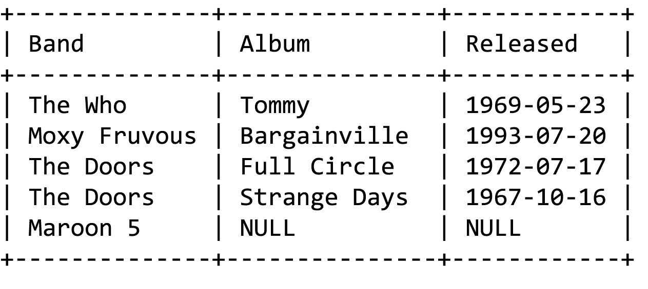
You may also be noticing that we still have not seen Maroon 5 come up in any of these examples, even though they were created when we first set up our bands table. That is because the basic join (also called “inner join”), as stated above, only returns results where records exist in both joined tables. Since we never added an album for Maroon 5, they did not come back as a result. We can capture all results of either table, and still pair them when records are available, by using different approaches to our join called left join and right join. Each of these performs roughly how it sounds—a left join will include all records from the left table, plus additional values from the right table when they exist, and a right join will do the opposite, including all the records from the right table and adding data from the left when it exists. Next we will look at all “Bands,” and any records they have, by using a left join. All we need to do is replace the comma between the tables in our “from” clause with the join method we want, and change the word “where” to “on”:
- Select bands.bandName as "Band", albums.albumName as "Album", releaseDate as "Released" from bands left join albums on albums.bandID=bands.bandID;
There are more complex forms of join than just left, right, and inner. However, these three cover most use cases and a well-designed database will usually reduce or eliminate the need for overly complex queries.
We can continue to add tables, and joins, to our queries to get more and more comprehensive results. We can even nest queries within one another inside sets of parenthesis. The query is then executed from the inside out just like it would in an equation, where the resulting data from the nested query is available to the query it sits inside of. First, we can look at a more complicated query that tells us everything about a particular song. We will specify a song title, and build a query that would connect all the related tables. Since our database is limited, we will start by looking at our table structure. If you want to fully test this example, you will need to spend some time populating your tables further. Since we will have a song title, and the question is what else we can glean, we will use all the keys that make sense in combination with a song title. Within the song table, we have albumID. That is relevant, as it tells us the album(s) the song has been released on. Now that we have at least one albumID, we can get from our “Albums” table to the band table and producer table as well. Tracing to these does not reveal any additional keys we can use, so without extra nested queries this is our reach:
|
Bands bandID |
Albums albumID |
Songs songID |
Concerts2Artists id |
||
|
Labels producerID |
Locations locID |
Artists artistID |
Venues venueID |
Concerts concertID |
Bands2Labels id |
We are able to connect data from half of our database (ignoring our reference tables) just from having a song title. This query could look like the following:
- Select bandName, albumName, releaseDate, title, length, producer from bands, albums, songs, labels where songs.albumID=albums.albumID and albums.bandID=bands.bandID and albums.producerID=labels.producerID;
Each pairing of fields in our where clause creates another join between tables. As our queries become more complex, you may find they take longer to run. This is because more data has to be reviewed, and more connections found, to create the resulting table. This is also the point where optimization techniques like indexing (automatically building trees in the database) and other more advanced MySQL tools will come into play.
Nested Queries
We can take the results of one query into consideration in another by nesting queries within one another using parenthesis. This will frequently come into play when we do not have a starting value for a question we want to ask. For example if we wanted to find the artist with the largest album in terms of tracks, we would break the goal down into its elements. First, we need to find which album has the highest track count, since we do not have a known value to search for:
- Select max(length) from songs;
This query looks at each record in the songs table and finds the one with the largest value. We could also have done this by sorting the table as descending on the tracks column, but since we are going to nest it we only want one value returned to keep things simpler. Our next step is to join the bandID value from albums to the id field in our bands table, in order to get our name:
- Select bandName from bands, albums, songs where songs.length= (select max(length) from songs) and songs.albumID=albums.albumID and albums.bandID=bands.bandID;
Nested queries are also a great place to use a few more methods to search with, namely ANY, IN, SOME, ALL and EXISTS. ANY and SOME are equivalent, and IN works the same as ANY when your comparison is strict equality (just =). What this means is that when we interact with the results of a nested query, we can look at each record returned as a match against our where clause. Let us look at some mock examples:
Get the name of every artist who has an album with the word “free” anywhere in the title:
- Select artistName from artists where artist.id = ANY (select artist.id from albums where album.title like "% Free %");
- Select artistName from artists where artist.id IN (select artist.id from albums where album.title like "% Free %");
- Select artistName from artists where artist.id = SOME (select artist.id from albums where album.title like "% Free %");
To understand where these verbs become different, we could ask the question of which album(s) contain a certain set of songs. In this case, our nested select would include the songs we are interested in. Here, using the verb ANY would return all albums that have one or more of the songs listed on their albums. If we changed to ALL, then we would only get albums where all of the values returned by our nested query existed on the album.
Learn more
Keywords, search terms: Nested queries, sql joins, indexing, mysql optimization
Jeff Atwood’s Joins Examples: http://www.codinghorror.com/blog/2007/10/a-visual-explanation-of-sql-joins.html
MySQL’s Nested Examples: http://dev.mysql.com/tech-resources/articles/subqueries_part_1.html