1.2: Modeling

When I say “modeling,” I’m talking about something like Figure 1.1. In the lower-left corner of the figure is the system, something in the real world we’re interested in. Often, it’s something complicated, so we have to decide which details can be left out; removing details is called abstraction.

Figure 1.1: The modeling process

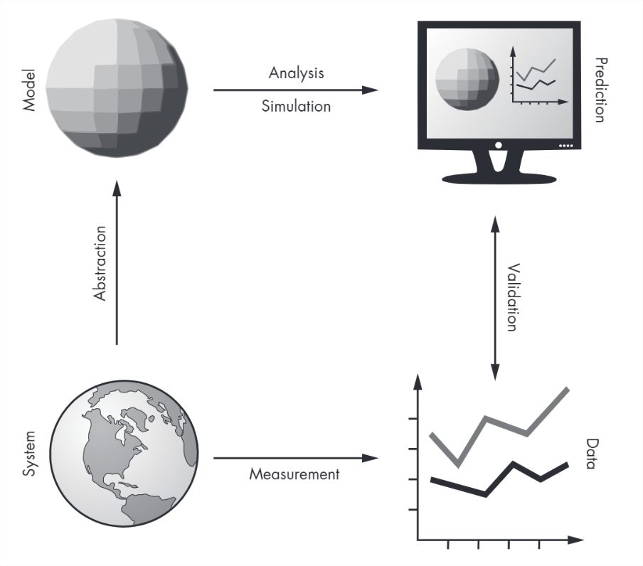
The result of abstraction is a model, shown in the upper left; a model is a description of the system that includes only the features we think are essential. A model can be represented in the form of diagrams and equations, which can be used for mathematical analysis. It can also be implemented in the form of a computer program, which can run simulations.

The result of analysis and simulation might be a prediction about what the system will do, an explanation of why it behaves the way it does, or a specific design engineered to satisfy a requirement or optimize performance.

We can validate predictions and test designs by taking measurements from the real world and comparing the data we get with the results from analysis and simulation.

For any physical system there are many possible models, each one including and excluding different features or including different levels of detail. The goal of the modeling process is to find the model best suited to its purpose (prediction, explanation, or design).

Sometimes the best model is the most detailed. If we include more features, the model is more realistic, and we expect its predictions to be more accurate. But often a simpler model is better. If we include only the essential features and leave out the rest, we get models that are easier to work with, and the explanations they provide can be clearer and more compelling.

As an example, suppose someone asked you why the orbit of the Earth is nearly elliptical. If you model the Earth and Sun as point masses (ignoring their actual size), compute the gravitational force between them using Newton’s law of universal gravitation, and compute the resulting orbit using Newton’s laws of motion, you can show that the result is an ellipse.

Of course, the actual orbit of Earth is not a perfect ellipse, because of the gravitational forces of the Moon, Jupiter, and other objects in the solar system, and because Newton’s laws of motion are only approximately true (they don’t take into account relativistic effects).

But adding these features to the model would not improve the explanation; more detail would only be a distraction from the fundamental cause. However, if the goal is to predict the position of the Earth with great precision, including more details might be necessary.

Choosing the best model depends on what the model is for. It is usually a good idea to start with a simple model, even if it’s likely to be too simple, and test whether it’s good enough for its purpose. Then you can add features gradually, starting with the ones you expect to be most essential. This process is called iterative modeling.

Comparing the results of successive models provides a form of internal validation so you can catch conceptual, mathematical, and software errors. And by adding and removing features, you can tell which ones have the biggest effect on the results, and which can be ignored. Comparing results with data from the real world provides external validation, which is generally the strongest test.

Figure 1.1 shows that models can be used for both analysis and simulation; in this book we will do some analysis, but the focus is on simulation. And the tool we will use to build simulations is MATLAB. So let’s get started.