
9.1: MATLAB Random Number Functions
- Page ID
- 83372

By Carey A. Smith
Random numbers are useful in MATLAB simulations of real-world signals and events which have uncertainty. There are 3 main MATLAB random number generators:
randi(IMAX,M,N) Random Integers
RndInt = randi(IMAX,M,N) returns an M-by-N matrix of uniformly distributed pseudo-random integers from 1 to IMAX.
Example 1A: Generate a vector of 8 dice rolls:
Dice = randi(6,1,8)
Example 1B: Generate a 4x3 array of random integers between 0 and 100
RndInt_4_3 = randi(100,4,3)
rand(M,N) Random Decimals
RndDec = rand(M,N) returns an M-by-N matrix of uniformly distributed pseudo-random decimal numbers between 0 and 1.
Example 2A: Generate 8 random decimals between 0 and 1:
RndDec2A = rand(1,8)
The vector can be scaled to be between any 2 numbers by adding an offset number and multiplying by a scale factor.
Example 2B: Generate 8 random decimals between –1 and 1:
RndDec2B = 2*rand(1,8) - 1
randn(M,N) Normally Distributed Random Numbers
RndNorm = randn(M,N) returns an M-by-N matrix of pseudo-random values drawn from the standard normal distribution, which has a mean (average) = 0 and a standard deviation = 1.
The standard deviation is a measure of the spread of the data. For a further explanation, watch this video:
“Standard Deviation - Explained and Visualized”, by Jeremy Blitz-Jones
https://www.youtube.com/watch?v=MRqtXL2WX2M
The Normal Distribution is also called the “Gaussian Distribution”.
Example 3A:
RndNorm3A = randn(1,5)
The result can be scaled to have any mean and standard deviation by adding an offset number and multiply by a scale factor.
% Example of randn() for pulse rates

% Generate a sample of 30 random pulse rates

% with a nominal mean = 90

% and a nominal standard deviation = 15.

n = 30

pmean    = 90

pstd_dev = 15

pulse = pmean + pstd_dev*randn(1,n); % This creates a 1xn vector
% Compute the sample mean and standard deviation.

pulse_mean = mean(pulse)

pulse_std = std(pulse)
%% Create a histogram of the results.

% For MATLAB use the histogram() function

% For Octave, use the older hist() function
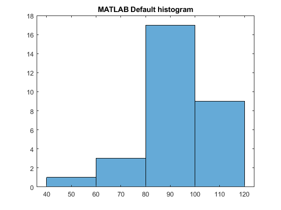
%% MATALB Default histogram

figure;

histogram(pulse)

title('MATLAB Default bins')
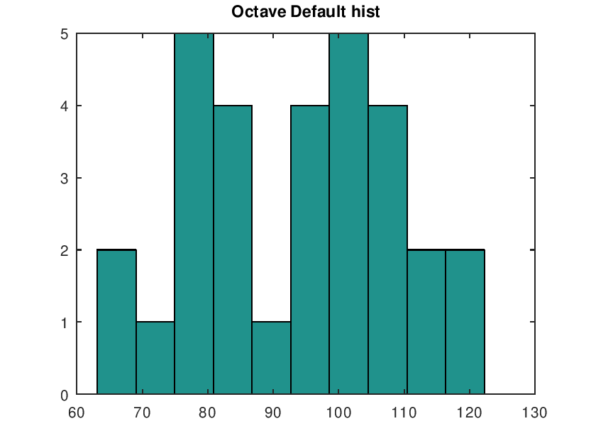
%% Octave Default histogram
graphics_toolkit("fltk") % Needed for Octave 7.2

figure;

hist(pulse)

title('Octave Default hist')
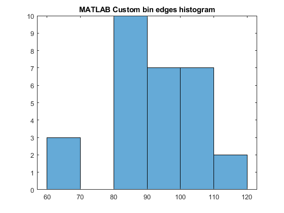
%% MATLAB Custom histogram

edges = 60 : 10 : 120;

figure;

histogram(pulse, edges)

title('MATLAB Custom bin edges histogram')
Solution
MATLAB Default
Octave:
MATLAB Custom bin edges
.
Example 3C: A radar signal has magnitude 20 with noise of magnitude = 4 (standard deviation)
Received_signal = 20 + 4*randn(1,5)
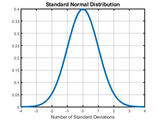
Figure \(\PageIndex{1}\): Standard Normal Probability Distribution
The total area under the curve = 1.00. Approximately:
68% is between -1 and +1 standard deviations
95% is between -2 and +2 standard deviations
99.7% is between -3 and +3 standard deviations
The normal distribution approximates many things, such as:
- Noise in signals
- Measurement errors
- Clinical trials of medicines and vaccines
- Probability and statistics
- Biological data, such as weights, heights, pulse rates, blood pressure, diabetes, etc.
The “Central Limit Theorem” states that the sum or average of random variables becomes normal as the number of data (the sample size) increases, even if the raw data is not normally distributed.
You may want to watch Mike’s Galton Machine video. It uses ball bearings to build up a normal distribution: https://www.youtube.com/watch?v=VQepRP-f6GA
See also: https://en.Wikipedia.org/wiki/Galton_board
The Standard Normal Probability Distribution plot can be created with this code:
% NormalDistribution.m
x = -4:0.01:4;
mu = 0; % mean
std_dev = 1; % standard deviation
y = (1/(std_dev*sqrt(2*pi))) * exp((-1/2)*((x-mu)/std_dev).^2);
figure;
plot(x,y,'LineWidth',4)
grid on;
title('Standard Normal Distribution','FontSize',14)
xlabel('Number of Standard Deviations','FontSize',12)
ax = gca
ax.LineWidth = 2