10.1.2: fzero() Examples and Exercises

fzero() is a "function of a function", because it needs a "handle" to a function that defines the equation whose root it will find. fzero() can be used either to find a zero of a single functions and or to find the intersection point of 2 functions.

Using fzero() to find the root of a single function

The way it works is as follows: It finds an interval containing the initial point. It uses nearby points to approximate derivatives and estimate where the zero is. It then re-evaluates the function at this new x value. It repeats this procedure until it finds a point where the function is zero or very nearly zero.

Example \(\PageIndex{1}\) Find a root of a 5th-order polynomial:

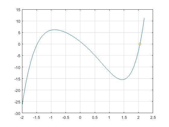
We will find a root of this 5th-order polynomial:

y = x.^5 - 4*x.^2 -10*x + 1;

Method 1: A straightforward way to do this is to create a function file for this:

% fpoly5.m:

function y = fpoly5(x)

y = x.^5 - 4*x.^2 -10*x + 1;

end

Create a separate m-file script (fzero_poly5.m) to visualize this function and to estimate the root.

%% A. Open a new figure and plot the function
x = -2:0.05:2.2;

y = fpoly5(x);

figure

plot(x,y)

grid on;

%% B. the value of x near x=2.1 that makes y = 0

x_solution = fzero(@fpoly5, 2.1) % @fpoly5 is a function "handle" to the file fpoly5.m

% fzero() evaluates the function fpoly5(x) multiple times, until it converges to a root. (A root is a value that makes the function = 0)

% x_solution = 2.0517

% Verify that this is a solution:

yb = fpoly5(x_solution)

% 7.1054e-15

hold on;

plot(x_solution,yb,'o')

----

Method 2: Another way is to create a local sub-function at the bottom of the m-file script. This method currently works in MATLAB, but not Octave.

Solution

.

Exercise \(\PageIndex{1}\) fzero_y_fun1

%% A. Create this function

function y1 = y_fun1(x)
y1 = log(x)./x.^2 -0.1;
end

Create a separate m-file script to visualize this function and to estimate the root.

%% B. (1 pt) In this 2nd file, create an x vector from 0.2 to 2.0
% Choose an increment for x, such that the plot will be smooth--that is, no visible straight lines.
x = 1: 0.1 :6;
% (1 pt) Evaluate the equation using your x vector
y1 = y_fun1(x);

%% C. (1 pt) Open figure and plot this function.
% A plot of the function lets us estimate a root.

figure(1)
plot(x,y1)
grid on;
title('fzero1root\_fcnfile\_example.m CSmith')
hold on;
plot(x,zeros(size(x)),'r') % Plot a line for y = 0
%% D. (4 pts) Use the fzero() function to find a root near x = 4

Solution

x_solution = fzero(@y_fun1, 4)
% @y_fun1 = "function handle" to y_fun1.m
% The function y_fun1(x) must have a single input variable.
% fzero chooses the values of x for computing the function
% x_solution = 3.5656

%% E. fzero() can also be used to find a root between 2 values
x_solution = fzero(@y_fun1, [3,5])

.

Exercise \(\PageIndex{2}\) fzero for y = log10(x) + 0.44;

%% Create a function m-file that computes y = log10(x) + 0.44;
% Set
x = 0 : 0.02 : 1;

Create a separate m-file script to visualize this function and to estimate the root.

% Compute y for this x vector using your function.
% Open a figure and plot(x, y)
% Turn the grid on

% Use fzero() to find a root near 0.4 of this function

Answer

Add texts here. Do not delete this text first.

.