16.2: Nonlinear Interpolation

A smoother interpolation than linear interpolation is called spline interpolation. Originally, a "spline" was a strip of flexible material that could be bent, so that a person could make a smooth curve through data points. The mathematical spline connects the data points with 3rd-order polynomial segments whose 1st and 2nd derivatives are continuous at each point. In MATLAB/Ocatave "spline" is an option with the interp1() function. The next example show how to use it and what the result is.

Example \(\PageIndex{1}\) Spline interpolation

This data is from Seimers example 40. It shows that the spline is smoother than the linear interpolation.

x1 = 0:5;
y1 = [12,10,9,6,2,0];
figure;
plot(x1, y1, 'o')
grid on

%% Interpolate with linear segments
x2 = 0: 0.1: 5; % Point spacing for plotting the fitted curve
% The default interpolation method is 'linear':
y2 = interp1(x1, y1, x2); % Compute the curve
hold on;
plot(x2, y2)
title('Interpolation with lines between the data points')

%% Interpolate with a smooth spline curve
y3 = interp1(x1, y1, x2, 'spline'); % Compute the curve with the 'spline' option
hold on;
plot(x2,y3,'r')
title('Interpolation')
legend('data', 'spline')

Solution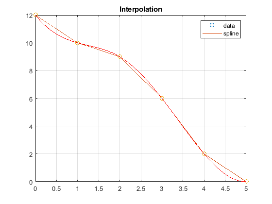

.

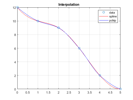
Another 3rd-order interpolation method in MATLAB is "pchip". The difference is the assumptions on the derivatives in the 2 end segments. The pchip is a newer algorithm and is often preferred over the spline.

Example \(\PageIndex{2}\) Pchip Interpolation

Pchip interpolation is compared to spline interpolation in this example, using the same data and spline as in the previous example.

figure;
plot(x1,y1,'o')
grid on
y3 = interp1(x1, y1, x2, 'spline'); % Compute the curve
hold on;
plot(x2,y3,'r')
title('Interpolation')

%% Interpolate with a smooth pchip fit
y3 = interp1(x1, y1, x2, 'pchip'); % Compute the curve with the 'pchip' option
plot(x2,y3,'b')
title('Interpolation')
legend('data', 'spline', 'pchip')
% 'pchip' and 'spline' only differ in the 2 end segments

Solution

.

Exercise \(\PageIndex{1}\) Nonlinear Interpolation Exercise1

Create an m-file script. Define this a, y data set:

x0 = -10:3:10;
y0 = -5 +2*x0 + 0.9*x0.^2 - 0.3*x0.^3;

Open a figure and plot this data using the 'o' marker. (No line)

Use hold on.

Define these x-points at which to compute the interpolated curves:

x2 = -10:0.5 : 10;

Interpolate the data from the x, y data to the x2 values with linear interpolation. Plot the result on the same figure.

Interpolate the data from the x, y data to the x2 values with spline interpolation. Plot the result on the same figure.

Interpolate the data from the x, y data to the x2 values with pchip interpolation. Plot the result on the same figure.

Add a legend and a title.

Answer

The solution is not given here.

There is also the interp2() function for doing interpolation on a 2-dimensional array of data.

Exercise \(\PageIndex{2}\) Nonlinear Interpolation Exercise2

Construct this data set:

x0 = -10:3:10;
y0 = -5 + 10*x0 - 2*x0.^3 + 0.1*x0.^4;

Open a figure.

Do the following interpolations and plot them on the same figure: Linear, spline, and pchip.

Add a legend.

Answer

The solution is not given here.

.

Exercise \(\PageIndex{3}\) Weather Temperature Interpolation

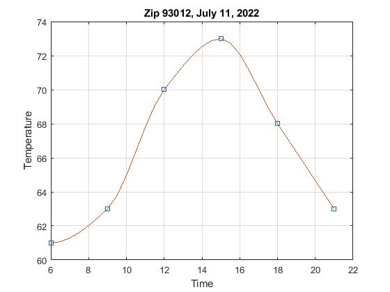
Go to weather.gov. Enter your zip code. Click on "3 Day History" (under "More Information") and find the temperatures for a recent day for every 3 hours from 6:00 to 21:00 (9 pm).

Open a new figure. Create and plot temperature vs. time (use 24 hour time) with the 's' marker. % (The x-axis is time, the y-axis is temperature.)

Add hold on to your .m file.

Create a new time vector from 6 to 21 with increments of 0.5 hours. Compute the pchip interpolation for this new time vector and plot it as a curve on the same plot.

Put a title with the zip code and the date of the data.

Label the x and y axes. Turn the grid on.

Answer

This is an example. Use your own data. Your data will be different.

..