18.2: Numerical Differentiation

1-Dimensional Derivatives

In calculus, you learned that the derivative of a function is: limit of Δy/Δx as x goes to 0.

Sometimes, we only have measured data, not an analytic function, so we cannot get the derivative analytically. When the analytic derivative is unknown, we can approximate it from the data using Δy/Δx, without taking a limit. The numerical derivative at point (xn, yn) is:

(xn, yn) ≈ (yn+1 – yn-1) / (xn+1 - xn-1,)

Matlab’s function for this is named gradient(). There are 2 methods of calling gradient(). Both methods take 2 arguments, and the 1st argument is the vector of y-values. The 2nd argument depends on the method:

Method A: dydx_gradient = gradient(y, x) where the 2nd argument is the vector of the x values corresponding to y.

Note: Both y and x need to be inputs.
When y is the only input, gradient(y) assumes that the x spacing = 1, which gives the wrong answer by a factor of 10!

Method B. dydx_gradient = gradient(y, dx), where the 2nd argument is the spacing, dx, between the x values (dx = a single number).

Both methods give the same results when the x values are equally spaced.

 

Example \(\PageIndex{1}\) Numerical Derivative of sin(x)

dx = 0.05*pi

x = 0: dx: 0.5*pi;

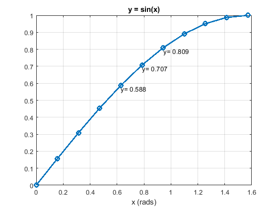
y = sin(x);

%% First, plot y vs. x
figure;
plot(x,y,'-o', 'LineWidth',2);
grid on;
title('y = sin(x)')
xlabel('x (rads)')

%% Label the (x, y) values of 3 consecutive points
text(x(5), (y(5)-0.02),['y= ',num2str(y(5),3)])
text(x(6), (y(6)-0.02),['y= ',num2str(y(6),3)])
text(x(7), (y(7)-0.02),['y= ',num2str(y(7),3)])

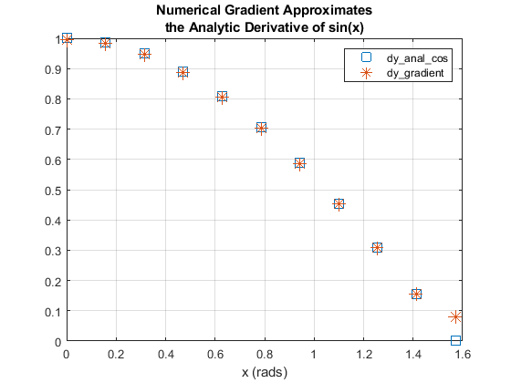
%% Second, plot the analytic derivative
dy_anal = cos(x); % This is the analytic derivative
figure;
%subplot(2,1,1);
plot(x,dy_anal,'s','MarkerSize',10);
grid on;
xlabel('x (rads)')

%% Approximate the derivative with the gradient function: grad()

dydx_gradientA = gradient(y, x) % Method A
dydx_gradientB = gradient(y, dx) % Method B

dydx_gradientA =
Columns 1 through 4
0.9959 0.9836 0.9472 0.8873
Columns 5 through 8
0.8057 0.7042 0.5854 0.4521
Columns 9 through 11
0.3077 0.1558 0.0784
dydx_gradientB =
Columns 1 through 4
0.9959 0.9836 0.9472 0.8873
Columns 5 through 8
0.8057 0.7042 0.5854 0.4521
Columns 9 through 11
0.3077 0.1558 0.0784

hold on;
plot(x, dydx_gradientA, '*', 'MarkerSize',10);
legend('dy\_anal\_cos','dy\_gradient')
title({'Numerical Gradient Approximates',
'the Analytic Derivative of sin(x)'})

Solution

.

Figure \(\PageIndex{1}\): y = sin(x)

Figure \(\PageIndex{1}\): Derivatives of y = sin(x) The numerical derivative is very close to the analytic values, except for the last point, because there is no point beyond the last point to improve the estimated value.

Add example text here.

.

Homework:

Exercise \(\PageIndex{2}\) Derivative of the normal distribution

Download the attached norm.m file which computes the normal distribution:

% Start a script .m file with this line:
clear all; close all; clc; format compact
% Define this vector
x = -3: 0.1 : 3;
% Compute y:
y = norm_dist(x);
%% Open a figure and plot y as a function of x:
% Turn on the grid:
%% Use gradient() to compute the derivative.
%% Then plot the gradient result on the same figure;
% If computed correctly:
% the derivative will be > 0 for x < 0
% the derivative will be = 0 for x = 0
% the derivative will be < 0 for x > 0
% Use the legend function to identify the 2 curves:
legend('norm\_dist', 'derivative')
% Add this title:
title('norm_dist and its derivative')

Answer

The answer is not given here.

.

2 Dimensional Derivatives

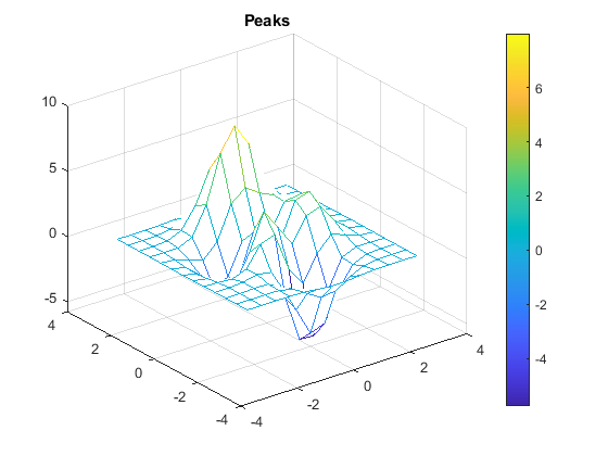
Matlab’s gradient function can also be used to compute the gradients of a function defined on x and y grids created by meshgrid. This example uses Matlab’s built-in peaks() 3D function.

Example \(\PageIndex{1}\)

%% Numerical Derivatives of the Peaks 2D function
clear all; close all; clc; format compact
dx = 0.5;
x1D = (-3: dx : 3);
y1D = x1D;
[x2Da, y2Da] = meshgrid(x1D,y1D);
[x2D, y2D, z2D] = peaks(x2Da,y2Da);
figure;
mesh(x2D, y2D, z2D)
title('Peaks')

colorbar
%%
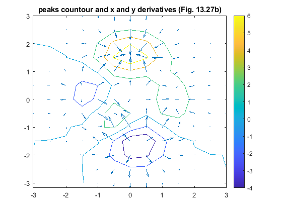
[dzdx, dzdy] = gradient(z2D, x1D, y1D);
figure;
contour(x2D, y2D, z2D);

axis equal
hold on;
% Draw the x & y cradients as arrows with the quiver plot function
quiver(x2D, y2D, dzdx, dzdy);
title('peaks countour and x and y derivatives (Fig. 13.27b)')

colorbar

Solution

The resulting plots are:

.