1.4: Internal Forces in Beams and Frames
- Page ID
- 17610

Internal Forces in Beams and Frames
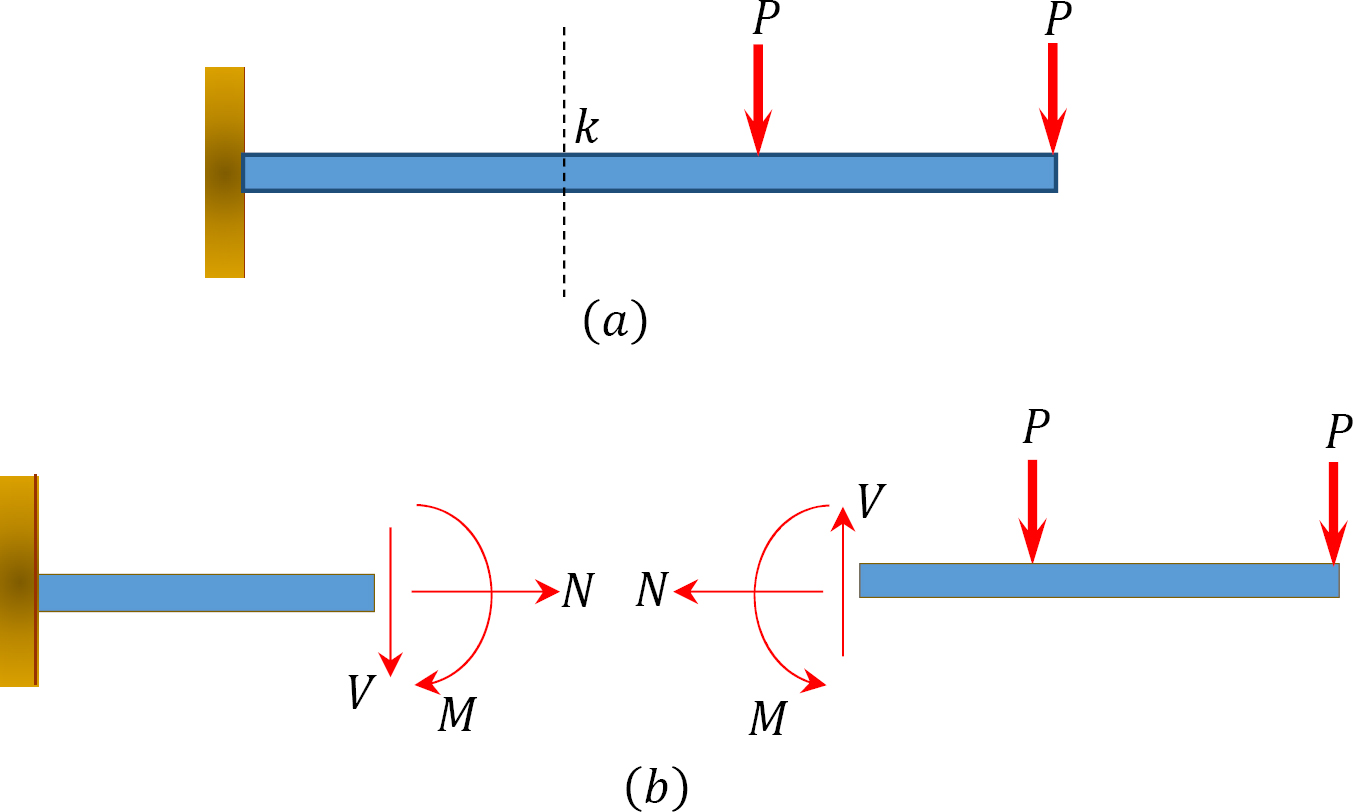
When a beam or frame is subjected to transverse loadings, the three possible internal forces that are developed are the normal or axial force, the shearing force, and the bending moment, as shown in section k of the cantilever of Figure 4.1. To predict the behavior of structures, the magnitudes of these forces must be known. In this chapter, the student will learn how to determine the magnitude of the shearing force and bending moment at any section of a beam or frame and how to present the computed values in a graphical form, which is referred to as the “shearing force” and the “bending moment diagrams.” Bending moment and shearing force diagrams aid immeasurably during design, as they show the maximum bending moments and shearing forces needed for sizing structural members.
4.2.1 Normal Force
The normal force at any section of a structure is defined as the algebraic sum of the axial forces acting on either side of the section.
4.2.2 Shearing Force
The shearing force (SF) is defined as the algebraic sum of all the transverse forces acting on either side of the section of a beam or a frame. The phrase “on either side” is important, as it implies that at any particular instance the shearing force can be obtained by summing up the transverse forces on the left side of the section or on the right side of the section.
4.2.3 Bending Moment
The bending moment (BM) is defined as the algebraic sum of all the forces’ moments acting on either side of the section of a beam or a frame.
4.2.4 Shearing Force Diagram
This is a graphical representation of the variation of the shearing force on a portion or the entire length of a beam or frame. As a convention, the shearing force diagram can be drawn above or below the x-centroidal axis of the structure, but it must be indicated if it is a positive or negative shear force.
4.2.5 Bending Moment Diagram
This is a graphical representation of the variation of the bending moment on a segment or the entire length of a beam or frame. As a convention, the positive bending moments are drawn above the x-centroidal axis of the structure, while the negative bending moments are drawn below the axis.
4.3.1 Axial Force
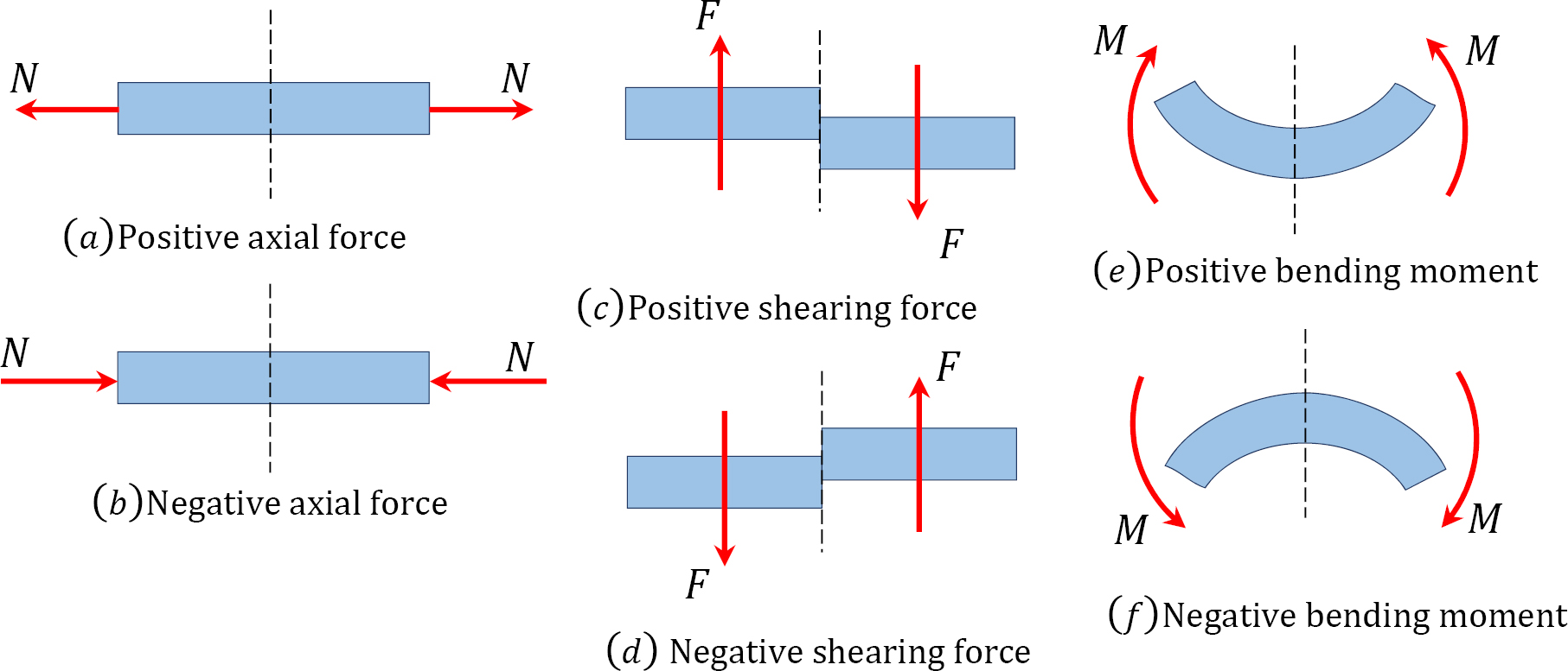
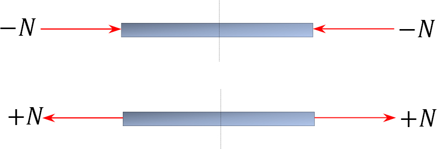
An axial force is regarded as positive if it tends to tier the member at the section under consideration. Such a force is regarded as tensile, while the member is said to be subjected to axial tension. On the other hand, an axial force is considered negative if it tends to crush the member at the section being considered. Such force is regarded as compressive, while the member is said to be in axial compression (see Figure 4.2a and Figure 4.2b).
4.3.2 Shear Force
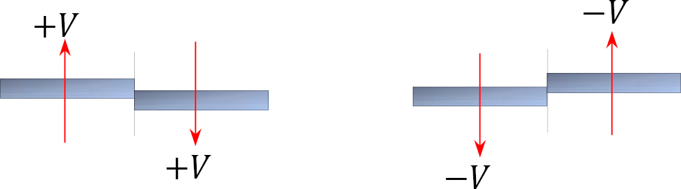
A shear force that tends to move the left of the section upward or the right side of the section downward will be regarded as positive. Similarly, a shear force that has the tendency to move the left side of the section downward or the right side upward will be considered a negative shear force (see Figure 4.2c and Figure 4.2d).
4.3.3 Bending Moment
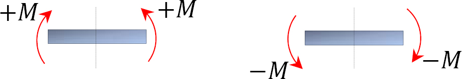
A bending moment is considered positive if it tends to cause concavity upward (sagging). If the bending moment tends to cause concavity downward (hogging), it will be considered a negative bending moment (see Figure 4.2e and Figure 4.2f).
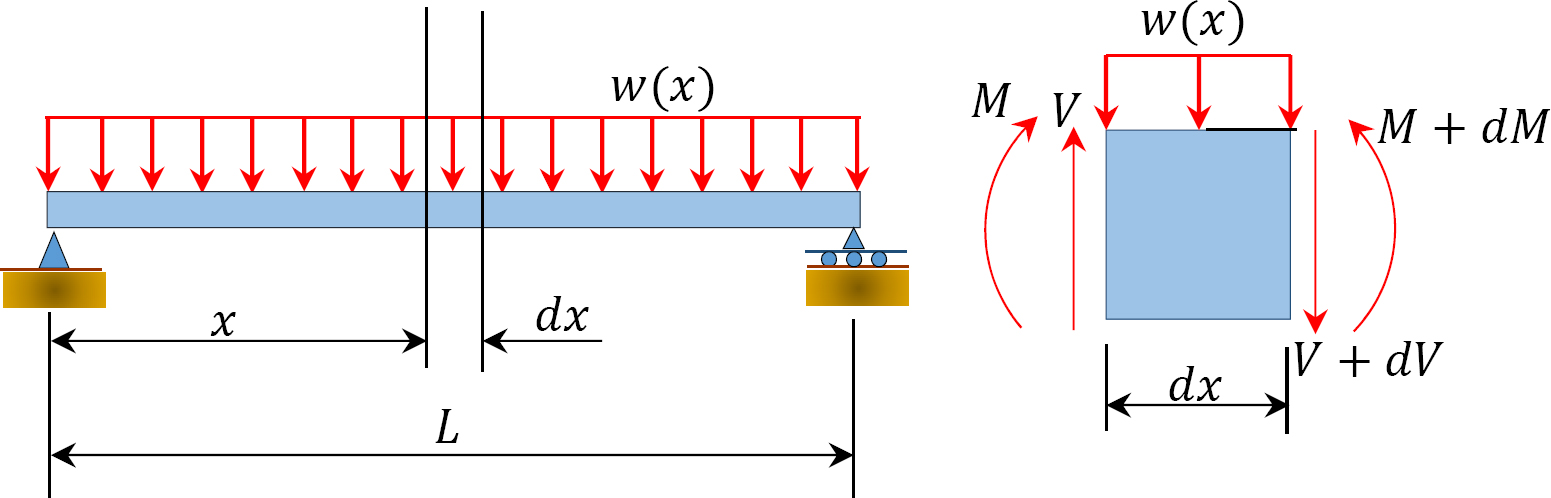
4.4 Relation Among Distributed Load, Shearing Force, and Bending Moment
For the derivation of the relations among w, V, and M, consider a simply supported beam subjected to a uniformly distributed load throughout its length, as shown in Figure 4.3. Let the shear force and bending moment at a section located at a distance of x from the left support be V and M, respectively, and at a section x + dx be V + dV and M + dM, respectively. The total load acting through the center of the infinitesimal length is wdx.
To compute the bending moment at section x + dx, use the following:
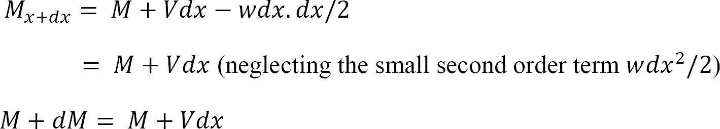

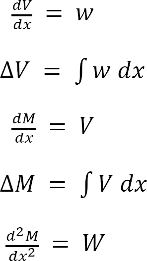
Equation 4.1 implies that the first derivative of the bending moment with respect to the distance is equal to the shearing force. The equation also suggests that the slope of the moment diagram at a particular point is equal to the shear force at that same point. Equation 4.1 suggests the following expression:

Equation 4.2 states that the change in moment equals the area under the shear diagram. Similarly, the shearing force at section x + dx is as follows:
Vx+dx = V – wdx
V + dV = V – wdx
or

Equation 4.3 implies that the first derivative of the shearing force with respect to the distance is equal to the intensity of the distributed load. Equation 4.3 suggests the following expression:

Equation 4.4 states that the change in the shear force is equal to the area under the load diagram. Equation 4.1 and 4.3 suggest the following:

Equation 4.5 implies that the second derivative of the bending moment with respect to the distance is equal to the intensity of the distributed load.
Procedure for Computation of Internal Forces
•Draw the free-body diagram of the structure.
•Check the stability and determinacy of the structure. If the structure is stable and determinate, proceed to the next step of the analysis.
•Determine the unknown reactions by applying the conditions of equilibrium.
•Pass an imaginary section perpendicular to the neutral axis of the structure at the point where the internal forces are to be determined. The passed section divides the structure into two parts. Consider either part of the structure for the computation of the desired internal forces.
•For axial force computation, determine the summation of the axial forces on the part being considered for analysis.
•For shearing force and bending moment computation, first write the functional expression for these internal forces for the segment where the section lies, with respect to the distance x from the origin.
•Compute the principal values of the shearing force and the bending moment at the segment where the section lies.
•Draw the axial force, shearing force, and bending moment diagram for the structure, noting the sign conventions discussed in section 4.3.
•For cantilevered structures, step three could be omitted by considering the free-end of the structure as the initial starting point of the analysis.
Example 4.1
Draw the shearing force and bending moment diagrams for the cantilever beam supporting a concentrated load at the free end, as shown in Figure 4.4a.
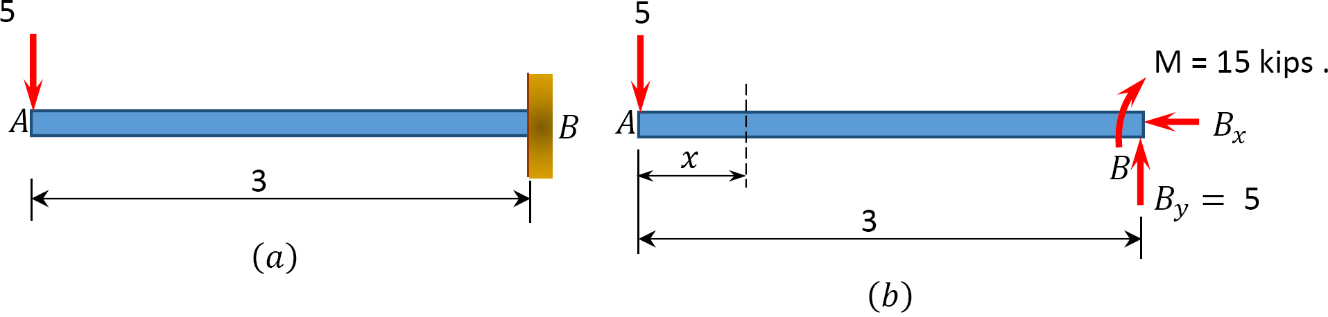
Solution
Support reactions. First, compute the reactions at the support. Since the support at B is fixed, there will be three reactions at that support, namely By, Bx, and MB, as shown in the free-body diagram in Figure 4.4b. Applying the conditions of equilibrium suggests the following:
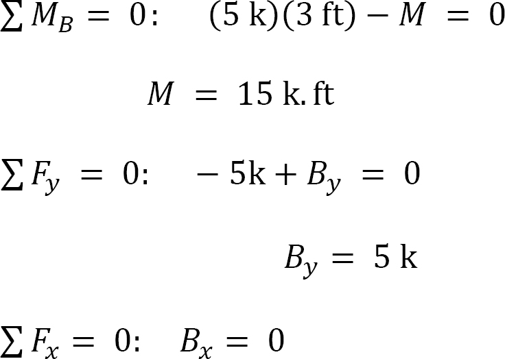
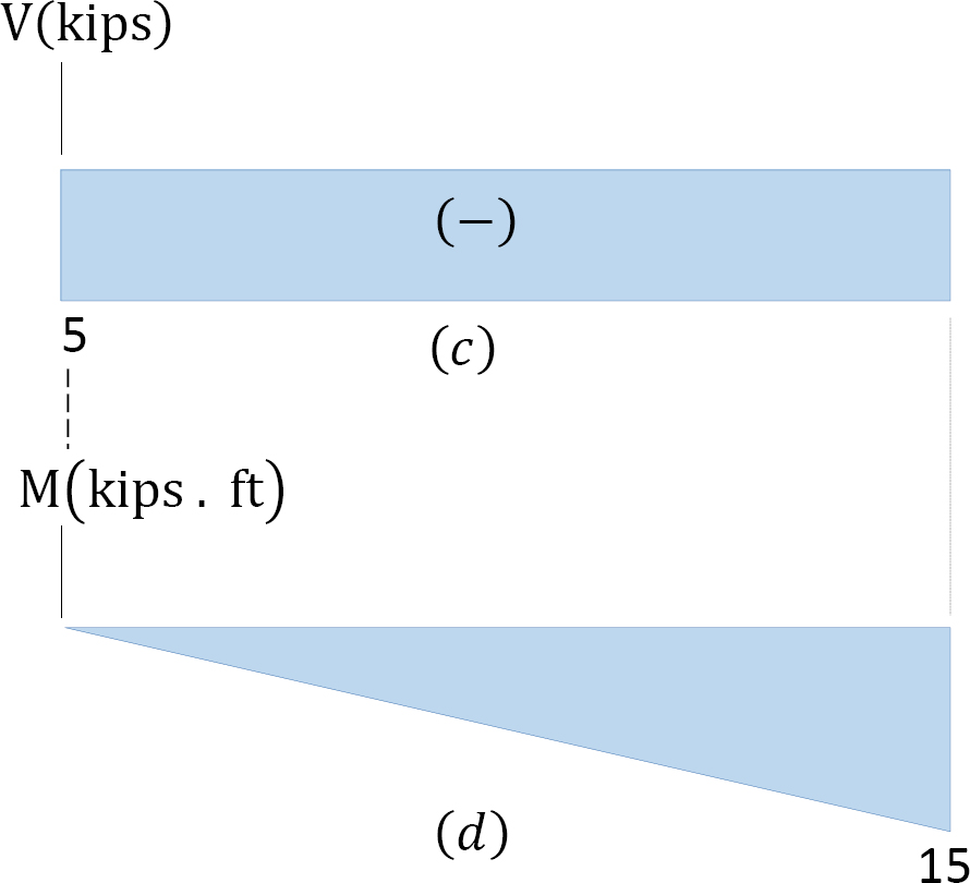
Shearing force (SF).
Shearing force function. Let x be the distance of an arbitrary section from the free end of the cantilever beam (Figure 4.4b). The shearing force at that section due to the transverse forces acting on the segment of the beam to the left of the section (see Figure 4.4e) is V = –5 k.
The negative sign is indicative of a negative shearing force. This is due to the fact that the sign convention for a shearing force states that a downward transverse force on the left of the section under consideration will cause a negative shearing force on that section.
Shearing force diagram. Note that because the shearing force is a constant, it must be of the same magnitude at any point along the beam. As a convention, the shearing force diagram is plotted above or below a line corresponding to the neutral axis of the beam, but a plus sign must be indicated if it is a positive shearing force, and a minus sign should be indicated if it is a negative shearing force, as shown in Figure 4.4c.
Bending moment (BM).
Bending moment function. By definition, the bending moment at a section is the summation of the moments of all the forces acting on either side of the section. Thus, the expression for the bending moment of the 5 k force on the section at a distance x from the free end of the cantilever beam is as follows:
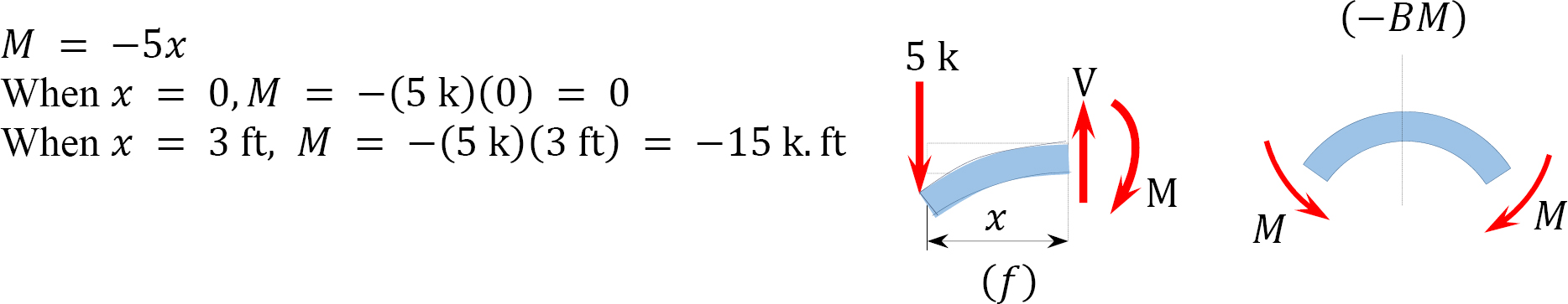
Bending moment diagram. Since the function for the bending moment is linear, the bending moment diagram is a straight line. Thus, it is enough to use the two principal values of bending moments determined at x = 0 ft and at x = 3 ft to plot the bending moment diagram. As a convention, negative bending moment diagrams are plotted below the neutral axis of the beam, while positive bending moment diagrams are plotted above the axis of the beam, as shown is Figure 4.4d.
Example 4.2
Draw the shearing force and bending moment diagrams for the cantilever beam subjected to a uniformly distributed load in its entire length, as shown in Figure 4.5a.
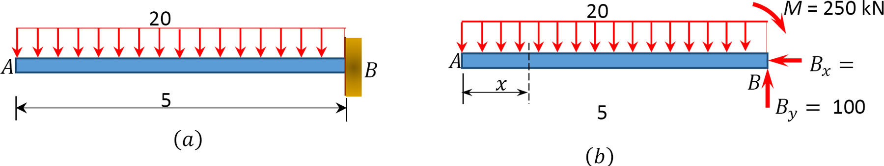
Solution
Support reactions. First, compute the reactions at the support. Since the support at B is fixed, there will possibly be three reactions at that support, namely By, Bx, and MB, as shown in the free-body diagram in Figure 4.4b. Applying the conditions of equilibrium suggests the following:

Shearing force (SF).
Shearing force function. Let x be the distance of an arbitrary section from the free end of the cantilever beam, as shown in Figure 4.5b. The shearing force of all the forces acting on the segment of the beam to the left of the section, as shown in Figure 4.5e, is determined as follows:

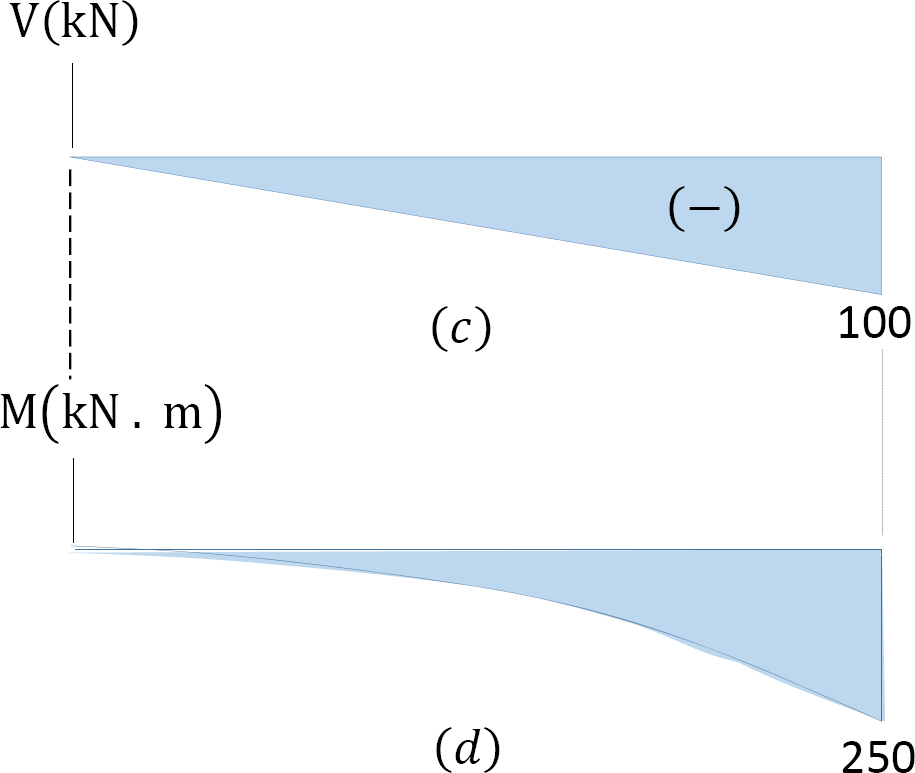
The obtained expression is valid for the entire beam. The negative sign indicates a negative shearing force, which was established from the sign convention for a shearing force. The expression also shows that the shearing force varies linearly with the length of the beam.
Shearing force diagram. Note that because the expression for the shearing force is linear, its diagram will consist of straight lines. The shearing force at x = 0 m and x = 5 m were determined and used for plotting the shearing force diagram, as shown in Figure 4.5c. As shown in the diagram, the shearing force varies from zero at the free end of the beam to 100 kN at the fixed end. The computed vertical reaction of By at the support can be regarded as a check for the accuracy of the analysis and diagram.
Bending moment (BM).
Bending moment expression. The expression for the bending moment at a section of a distance x from the free end of the cantilever beam is as follows:

Bending moment diagram. Since the function for the bending moment is parabolic, the bending moment diagram is a curve. In addition to the two principal values of bending moment at x = 0 m and at x = 5 m, the moments at other intermediate points should be determined to correctly draw the bending moment diagram. The bending moment diagram of the beam is shown in Figure 4.5d.
Example 4.3
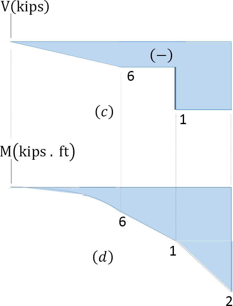
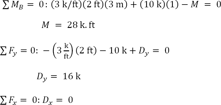
Draw the shearing force and bending moment diagrams for the cantilever beam subjected to the loads shown in Figure 4.6a.
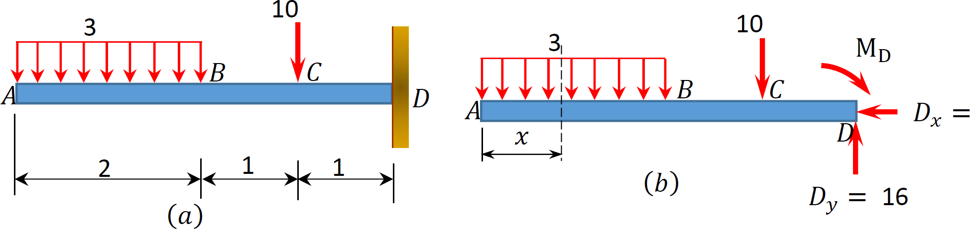
Solution
Support reactions. The free-body diagram of the beam is shown in Figure 4.6b. First, compute the reactions at the support B. Applying the conditions of equilibrium suggests the following:
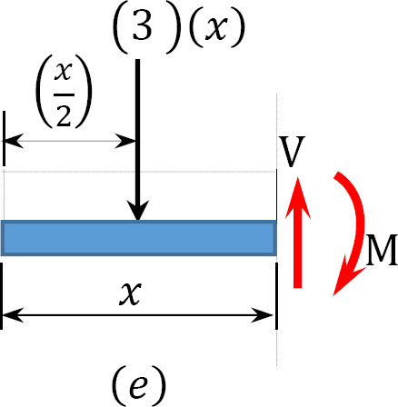
Shearing force and bending moment functions. Due to the discontinuity of the distributed load at point B and the presence of the concentrated load at point C, three regions describe the shear and moment functions for the cantilever beam. The functions and the values for the shear force (V) and the bending moment (M) at sections in the three regions at a distance x from the free-end of the beam are as follows:
Segment AB 0 < x < 2 ft
V = −3x
When x = 0, V = 0
When x = 1, V = −3 kip
When x = 2 ft, V = −6 kip
When x = 0, M = 0
When x = 1 ft, M = −1.5 kip. ft
When x = 2 ft, M = −6 kip. ft
Segment BC 2 ft < x < 3 ft
V = −3(2) = −6 kip
When x = 2 ft, M = −6 kip. ft
When x = 3 ft, M = −12 kip. ft
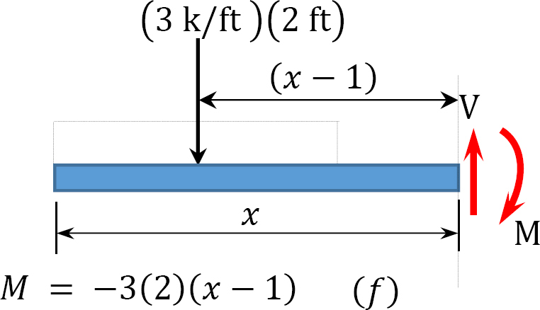
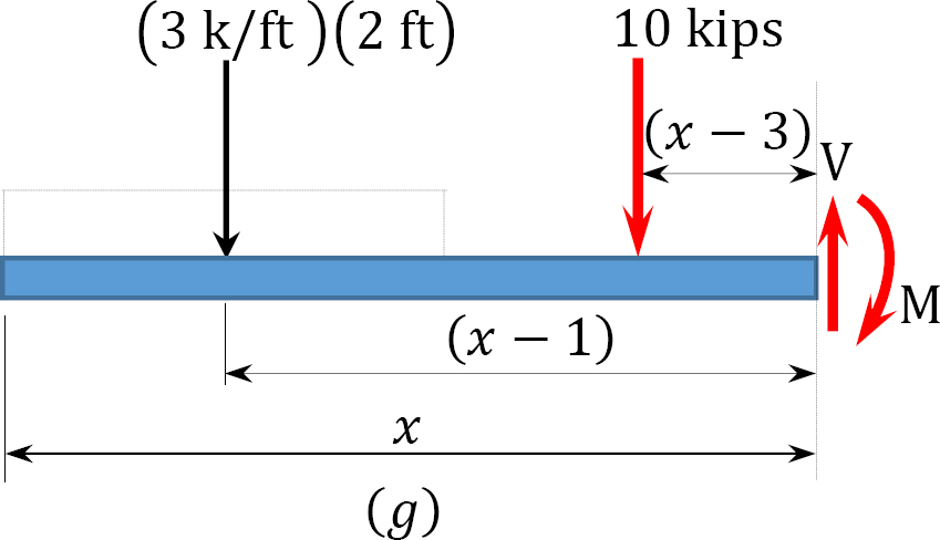
Segment CD 3 ft < x < 4 ft
V = −(3)(2) − 10 = −16 kips
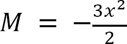
M = −(3)(2)(x − 1) − 10(x− 3)
When x = 3 ft, M = −12 kip. ft
When x = 4 ft, M = −28 kip. ft
Shearing force and bending moment diagrams. The computed values of the shearing force and bending moment are plotted in Figure 4.6c and Figure 4.6d. It is important to remember that there will always be a sudden change in the shearing force diagram where there is a concentrated load in the beam. The numerical value of the change should be equal to the value of the concentrated load. For instance, at point C where the concentrated load of 10 kips is located in the beam, the change in shearing force in the shear force diagram is 16 k - 6k = 10 kips. The bending moment diagram is a curve in portion AB and is straight lines in segments BC and CD.
Example 4.4
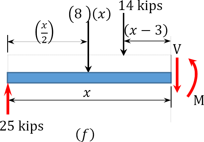
Draw the shearing force and bending moment diagrams for the beam with an overhang subjected to the loads shown in Figure 4.7a.
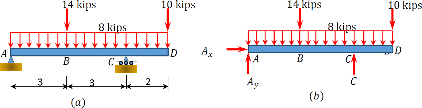
Solution
Support reactions. The reactions at the supports are shown in the free-body diagram of the beam in Figure 4.7b. They are computed by applying the conditions of equilibrium, as follows:
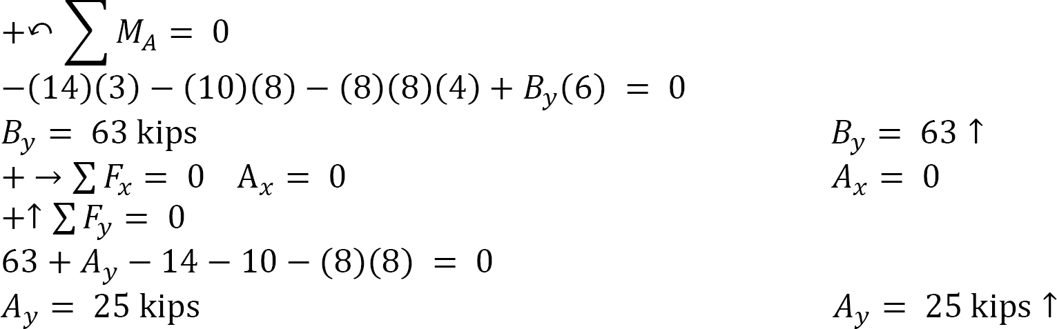
Shear and bending moment functions. Due to the concentrated load at point B and the overhanging portion CD, three regions are considered to describe the shearing force and bending moment functions for the overhanging beam. The expression for these functions at sections within each region and the principal values at the end points of each region are as follows:
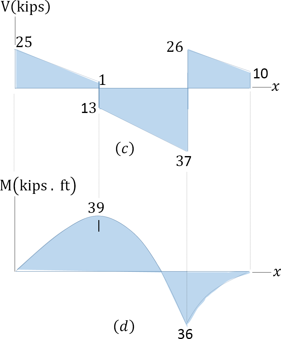
0 < x < 3
V = 25 − 8x
When x = 0, V = 25 kips
When x = 3, V = 1 kip
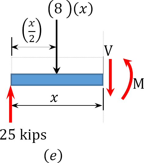
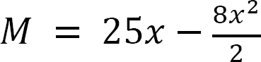
When x = 0, M = 0
When x = 3, M = 39 kip. ft
3 < x < 6
V = 25 − 14 − 8x
When x = 3, V = −13 kips
When x = 6, V = −37 kips
M = 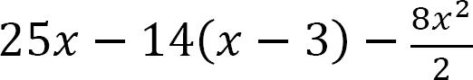
When x = 3, M = 39 k. ft
When x = 6, M = −36 kip. ft
0 < x < 2
V = 10 + 8x
When x = 0, V = 10 kips
When x = 2, V = 26 kips
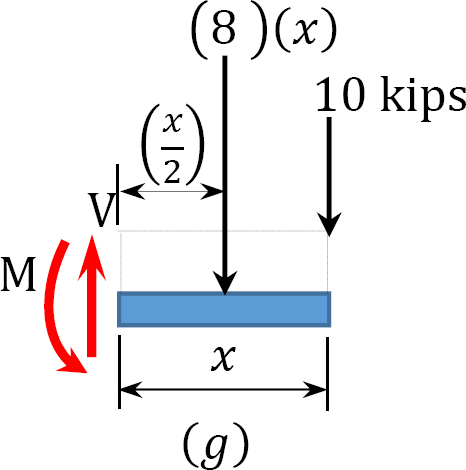
M = 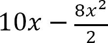
When x = 0, M = 0
When x = 2, M = −36 kip. ft
Shearing force and bending moment diagram. The determined shearing force and moment diagram at the end points of each region are plotted in Figure 4.7c and Figure 4.7d. For accurate plotting of the bending moment curve, it is sometimes necessary to determine some values of the bending moment at intermediate points by inserting some distances within the region into the obtained function for that region. Notice that at the location of concentrated loads and at the supports, the numerical values of the change in the shearing force are equal to the concentrated load or reaction.
Example 4.5
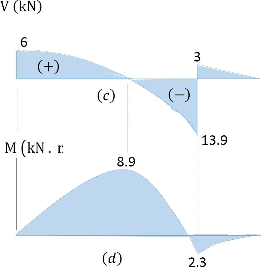
Draw the shearing force and bending moment diagrams for the beam with an overhang subjected to the loads shown in Figure 4.8a. Determine the position and the magnitude of the maximum bending moment.
Solution
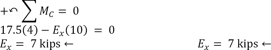
Support reactions. The reactions at the supports of the beam are shown in the free-body diagram in Figure 4.8b. The reactions are computed by applying the following equations of equilibrium:
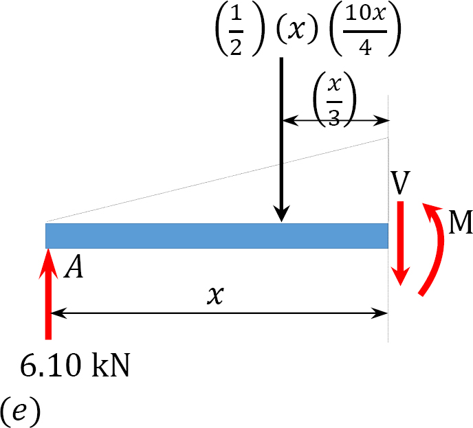
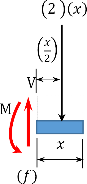
Shear and bending moment functions. Due to the discontinuity in the shades of distributed loads at the support B, two regions of x are considered for the description and moment functions, as shown below:
0 < x < 4
V = 
When x = 0, V = 6.10 kN
When x = 2, V = 1.1 kN
When x = 4, V = −13.9 kN
M = 
When x = 0, M = 0
When x = 2, M = 8.87 kN. m
When x = 4, M = −2.3 kN. m
0 < x < 1.5
V = 2x
When x = 0, V = 0
When x = 1.5, V = 3 kN
M = −(2)(x) 
When x = 0, M = 0
When x = 1.5 m, M = −2.3 kN. m
Position and magnitude of maximum bending moment. Maximum bending moment occurs where the shearing force equals zero. As shown in the shearing force diagram, the maximum bending moment occurs in the portion AB. Equating the expression for the shear force for that portion as equal to zero suggests the following:
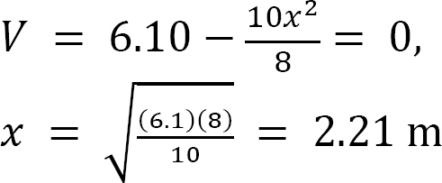
The magnitude of the maximum bending moment can be determined by putting x = 2.21 m into the expression for the bending moment for the portion AB. Thus,

Example 4.6
Draw the shearing force and bending moment diagrams for the compound beam subjected to the loads shown in Figure 4.9a.
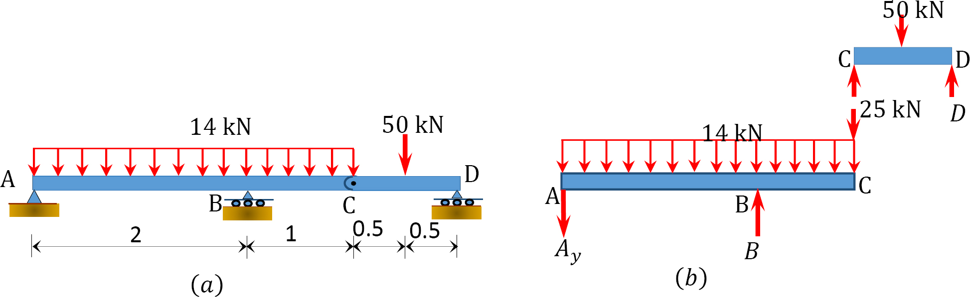
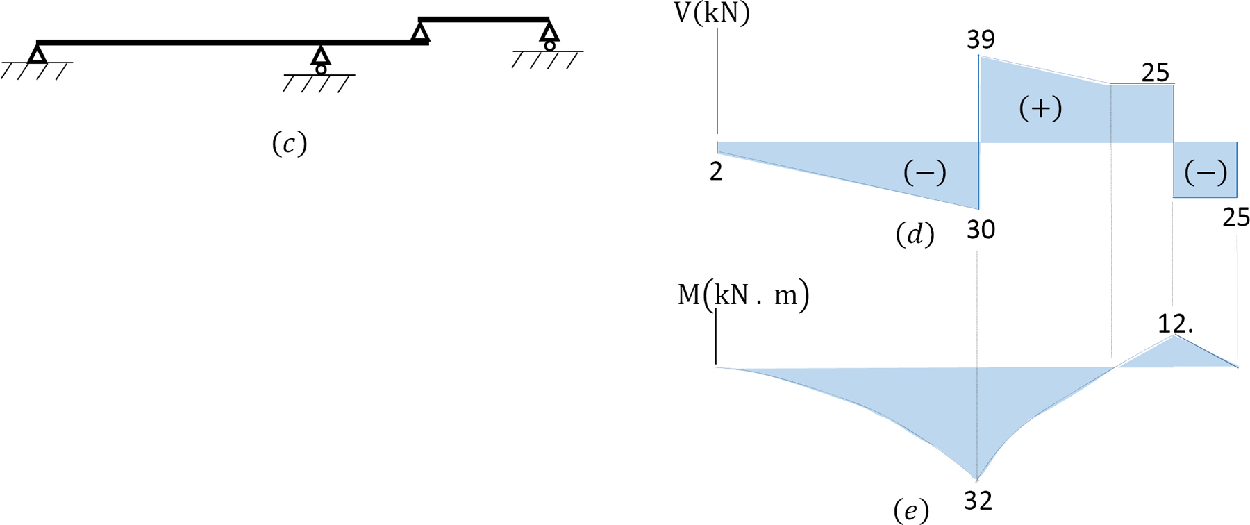
Solution
Free-body diagram. The free-body diagram of the beam is shown in Figure 4.9b.
Classification of structure. The compound beam has r = 4, m = 2, and fi = 2. Since 4 + 2 = 3(2), the structure is statically determinate.
Identification of the primary and complimentary structure. The schematic diagram of member interaction for the beam is shown in Figure 4.9c. The part AC is the primary structure, while part CD is the complimentary structure.
Analysis of complimentary structure.
Support reaction.
Cy = Dy = 25 kN, due to symmetry of loading.
Shear force and bending moment.
0 < x < 0.5
V = 25 kN
M = 25x
When x = 0, M = 0
When x = 0.5, M = 12.5 kN. m
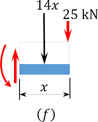
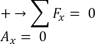
Analysis of primary structure.
Support reactions.
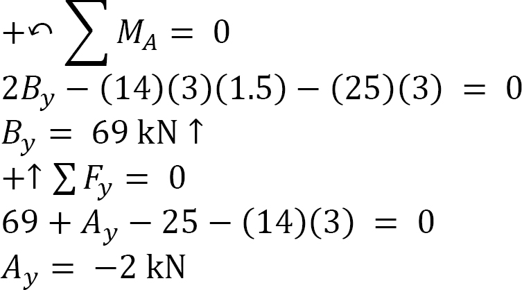
The negative implies the reaction at A acts downward.
Shear force and bending moment functions.
0 < x < 1
V = 25 + 14x
When x = 0, V = 25 kN
When x = 1, V = 39 kN
M = 
When x = 0, M = 0
When x = 1, M = −32 kN. m
0 < x < 2
V = −2 − 14x
When x = 0, V = −2 kN
When x = 2, V = −30 kN
M = 
When x = 0, M = 0
When x = 2, M = −32 kN. m
Example 4.7
Draw the shear force and bending moment diagrams for the frame subjected to the loads shown in Figure 4.10a.
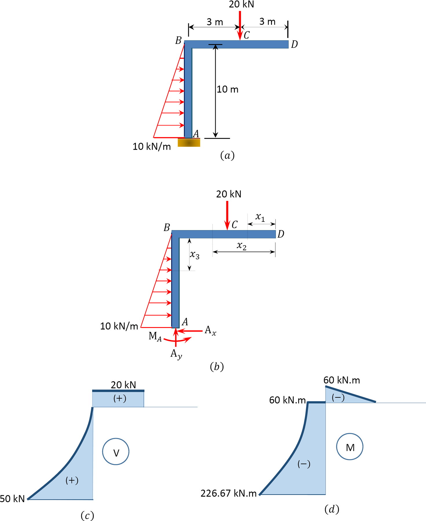
Solution
Free-body diagram. The free-body diagram of the beam is shown in Figure 4.10a.
Support reactions. The reactions at the support of the beam can be computed as follows when considering the free-body diagram and using the equations of equilibrium:
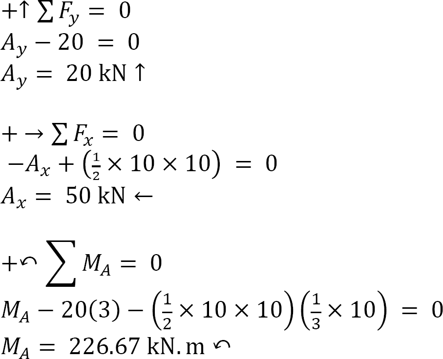
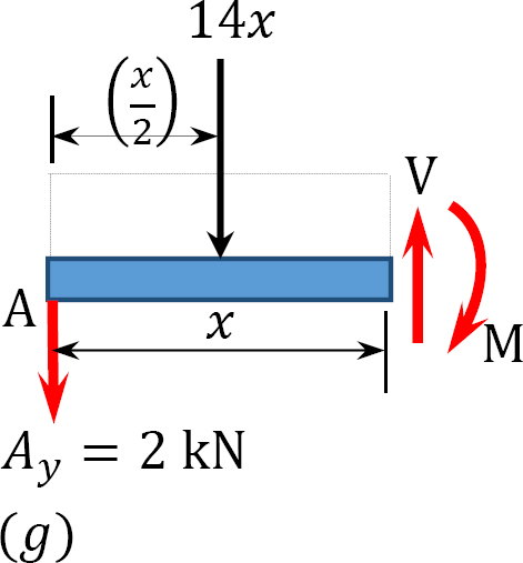
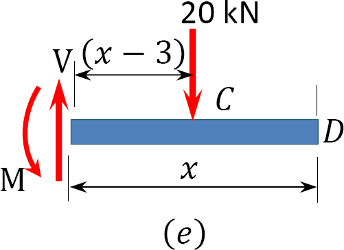
Shearing force and bending moment functions of beam BC.
0 < x1 < 3
V = 0
M = 0
3 < x2 < 6
V = 20 kN
M = −20 (x − 3)
When x = 3, M = 0
When x = 6, M = −60 kN. m
Note that the distance x to the section in the expressions is from the right end of the beam.
Shearing force and bending moment functions of column AB.
0 < x3 < 10
V 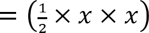
When x = 0, V = 0
When x = 10, V = 50 kN
M = 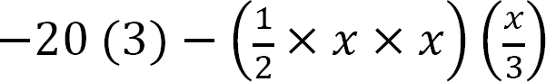
When x = 0, M = −60 kN. m
When x = 10, M = −226.67 kN. m
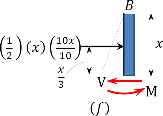
Note that the distance x to the section on the column is from the top of the column and that a similar triangle was used to determine the intensity of the triangular loading at the section in the column, as follows: 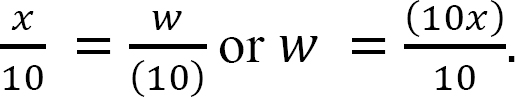
Shearing force and bending moment diagrams. The computed values of the shearing force and bending moment for the frame are plotted as shown in Figure 4.10c and Figure 4.10d.
Example 4.8
Draw the shearing force and bending moment diagrams for the frame subjected to the loads shown in Figure 4.11a.
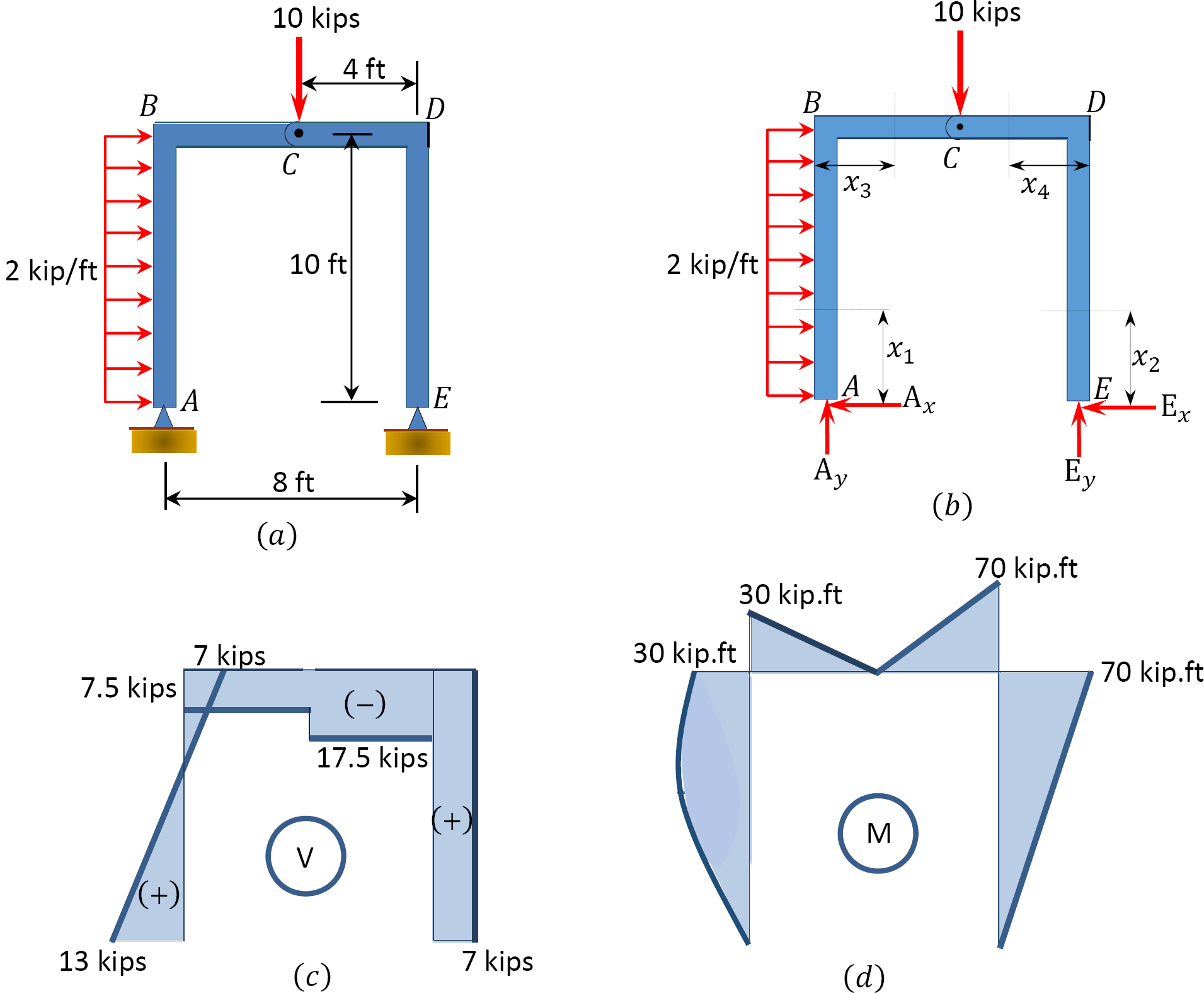
Solution
Free-body diagram. The free-body diagram of the beam is shown in Figure 4.11b.
Support reactions. The reactions at the supports of the frame can be computed by considering the free-body diagram of the entire frame and part of the frame. The vertical reactions of the supports at points A and E are computed by considering the equilibrium of the entire frame, as follows:
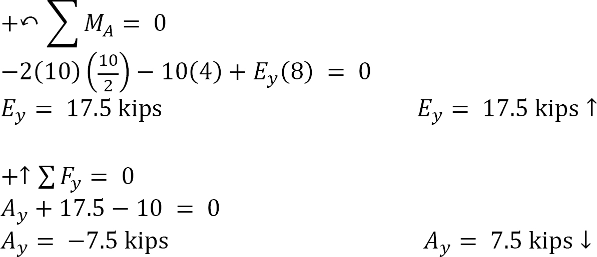
The negative sign indicates that Ay acts downward instead of upward as originally assumed.
Considering the equilibrium of part CDE of the frame, the horizontal reaction of the support at E is determined as follows:
Again, considering the equilibrium of the entire frame, the horizontal reaction at A can be computed as follows:
Shear and bending moment of the columns of the frame.
Shear force and bending moment in column AB.
0 < x1 < 10 ft
V = 13 − 2x
When x = 0, V = 13 kips
When x = 10 ft, V = −7 kips
M = 
When x = 0, M = 0
When x = 10 ft, M = 30 kip. ft
When x = 5 ft, M = 30 kip. ft
Shear force and bending moment in column ED.
0 < x2 < 10 ft
V = 7 kips
M = 7x
When x = 0, M = 0
When x = 10 ft, M = 70 kip. ft
Shear and bending moment of the frame’s beam.
Shear force and bending moment in beam BC.
0 < x3 < 4 ft
V = −7.5 kips
M = −7.5x + 13(10) − 2(10) 
When x = 0, M = 30 kip.ft
When x = 4 ft, M = 0
Shear force and bending moment in beam CD.
0 < x4 < 4 ft
V = −17.5 kips
M = 17.5x − 7(10)
When x = 0, M = −70 kip.ft
When x = 4 ft, M = 0
The computed values of the shearing force and bending moment for the frame are plotted in Figure 4.11c and Figure 4.11d.
Chapter Summary
Internal forces in beams and frames: When a beam or frame is subjected to external transverse forces and moments, three internal forces are developed in the member, namely the normal force (N), the shear force (V), and the bending moment (M). These are shown in the following Figure.
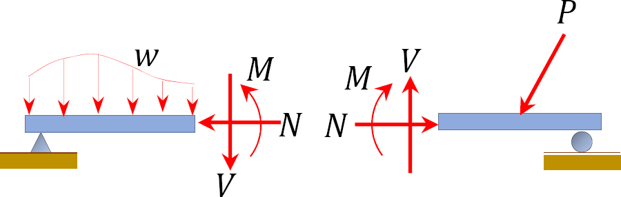
Normal force: The normal force at any section of a beam can be determined by adding up the horizontal, normal forces acting on either side of the section. If the resultant of the normal force tends to move towards the section, it is regarded as compression and is denoted as negative. However, if it tends to move away from the section, it is regarded as tension and is denoted as positive.
Shear force: The shear force at any section of a beam is determined as the summation of all the transverse forces acting on either side of the section. The sign convention adopted for shear forces is below. A diagram showing the variation of the shear force along a beam is called the shear force diagram.
Bending moment: The bending moment at a section of a beam can be determined by summing up the moment of all the forces acting on either side of the section. The sign convention for bending moments is shown below. A graphical representation of the bending moment acting on the beam is referred to as the bending moment diagram.
Relationship among distributed load, shear force, and bending moment: The following relationship exists among distributed loads, shear forces, and bending moments.
Practice Problems
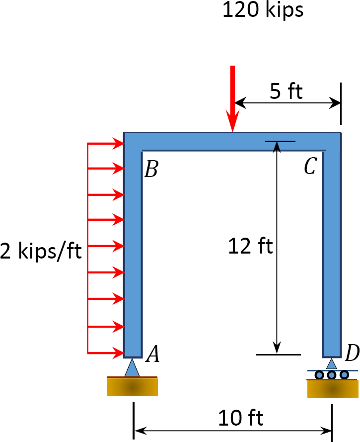
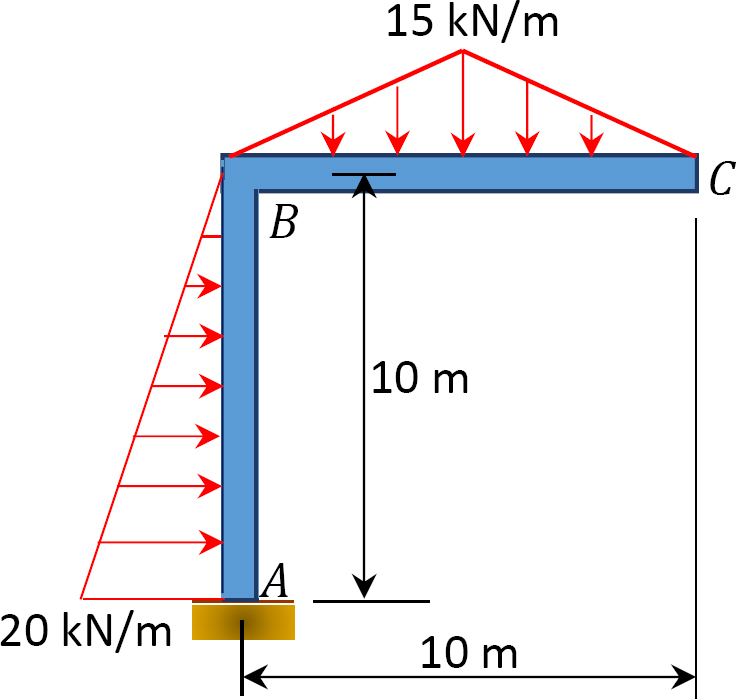
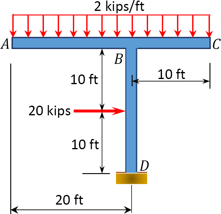
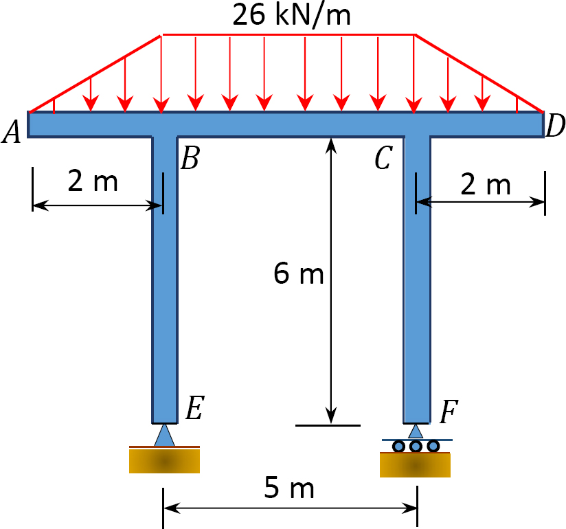
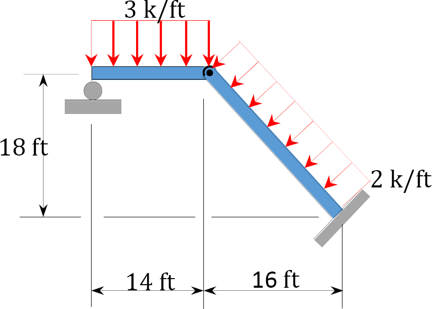
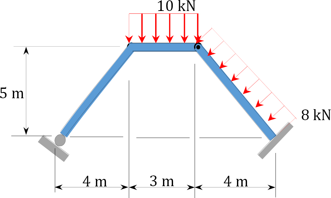
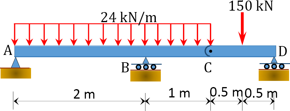
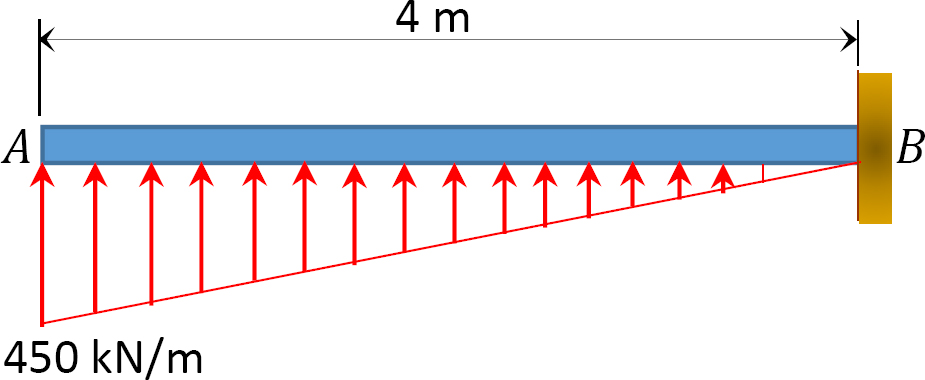
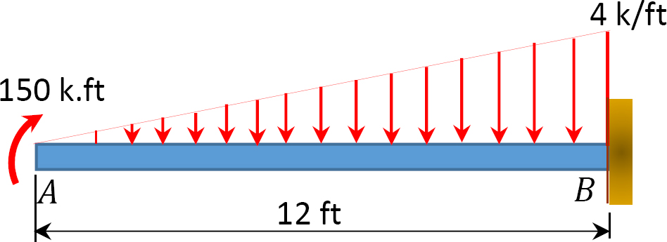
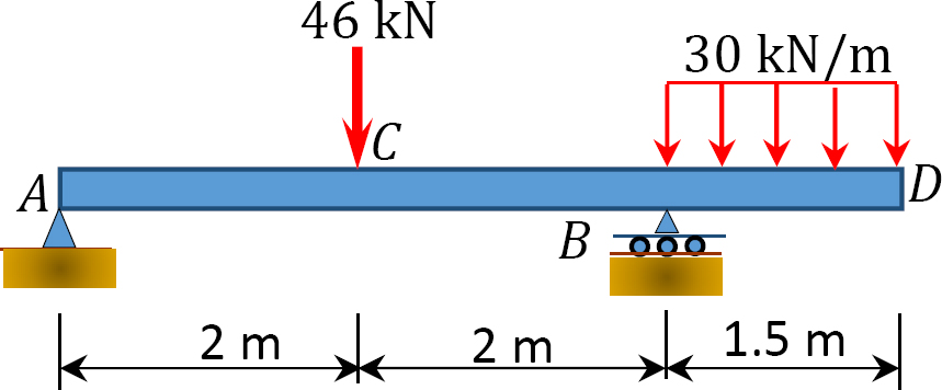
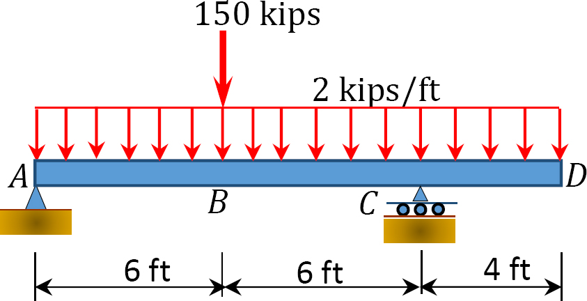
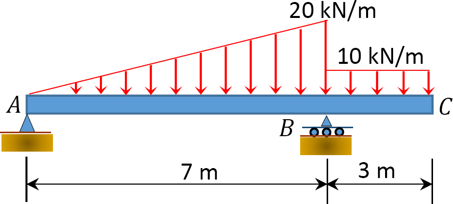
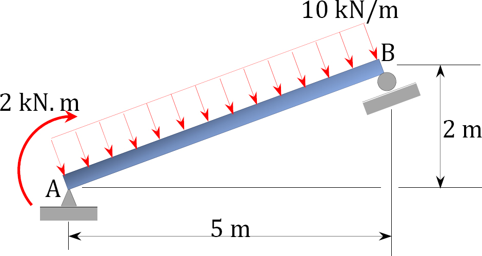
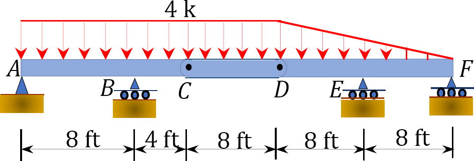
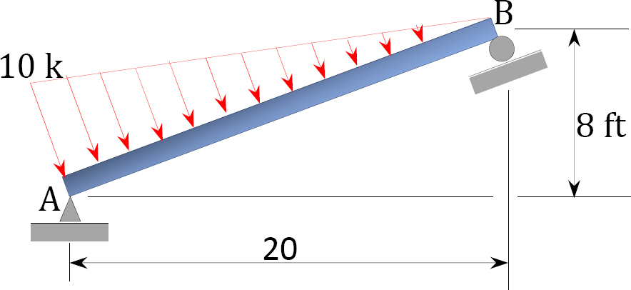
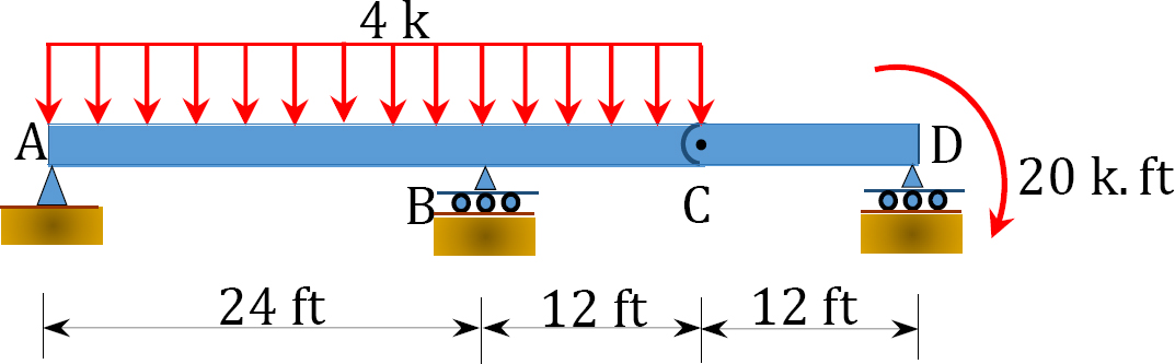
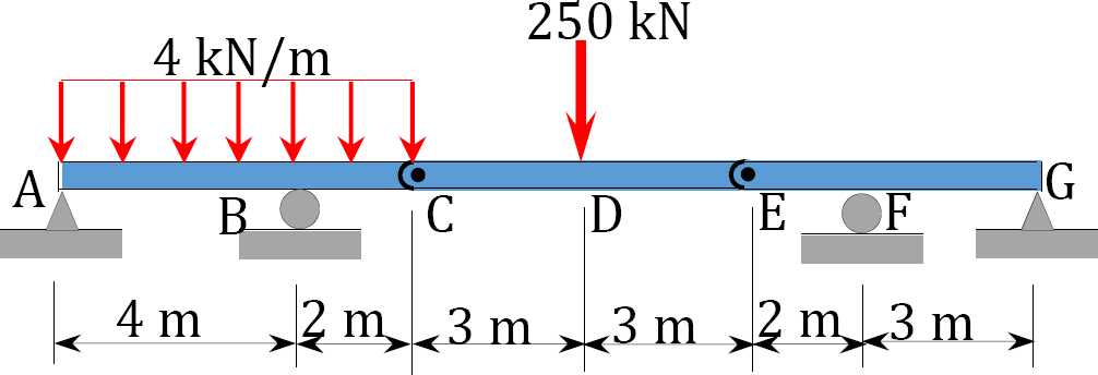
4.1. Draw the shearing force and the bending moment diagrams for the beams shown in Figure P4.1 through Figure P4.11.
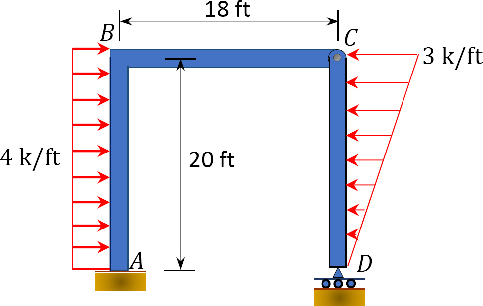
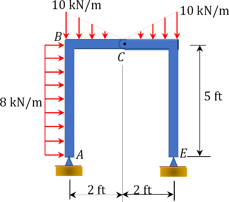
4.2. Draw the shearing force and the bending moment diagrams for the frames shown in Figure P4.12 through Figure P4.19.