1.2.1: Interpolation of Univariate Functions

The objective of interpolation is to approximate the behavior of a true underlying function using function values at a limited number of points. Interpolation serves two important, distinct purposes throughout this book. First, it is a mathematical tool that facilitates development and analysis of numerical techniques for, for example, integrating functions and solving differential equations. Second, interpolation can be used to estimate or infer the function behavior based on the function values recorded as a table, for example collected in an experiment (i.e., table lookup).

Let us define the interpolation problem for an univariate function, i.e., a function of single variable. We discretize the domain \(\left[x_{1}, x_{N}\right]\) into \(N-1\) non-overlapping segments, \(\left\{S_{1}, \ldots, S_{N-1}\right\}\), using \(N\) points, \(\left\{x_{1}, \ldots, x_{N}\right\}\), as shown in Figure 2.1. Each segment is defined by \[S_{i}=\left[x_{i}, x_{i+1}\right], \quad i=1, \ldots, N-1,\] and we denote the length of the segment by \(h\), i.e. \[h \equiv x_{i+1}-x_{i} .\] For simplicity, we assume \(h\) is constant throughout the domain. Discretization is a concept that is used throughout numerical analysis to approximate a continuous system (infinite-dimensional problem) as a discrete system (finite-dimensional problem) so that the solution can be estimated using a computer. For interpolation, discretization is characterized by the segment size \(h\); smaller \(h\) is generally more accurate but more costly.

Suppose, on segment \(S_{i}\), we are given \(M\) interpolation points \[\bar{x}^{m}, \quad m=1, \ldots, M\]

Figure 2.1: Discretization of a 1-D domain into \(N-1\) segments.

(a) discretization

(b) local interpolation

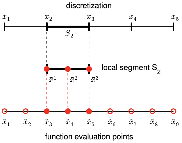
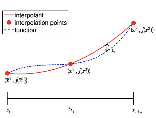
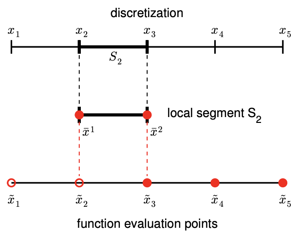
Figure 2.2: Example of a 1-D domain discretized into four segments, a local segment with \(M=3\) function evaluation points (i.e., interpolation points), and global function evaluation points (left). Construction of an interpolant on a segment (right).

and the associated function values \[f\left(\bar{x}^{m}\right), \quad m=1, \ldots, M\] We wish to approximate \(f(x)\) for any given \(x\) in \(S_{i}\). Specifically, we wish to construct an interpolant If that approximates \(f\) in the sense that \[(\mathcal{I} f)(x) \approx f(x), \quad \forall x \in S_{i},\] and satisfies \[(\mathcal{I} f)\left(\bar{x}^{m}\right)=f\left(\bar{x}^{m}\right), \quad m=1, \ldots, M .\] Note that, by definition, the interpolant matches the function value at the interpolation points, \(\left\{\bar{x}^{m}\right\}\).

The relationship between the discretization, a local segment, and interpolation points is illustrated in Figure 2.2(a). The domain \(\left[x_{1}, x_{5}\right]\) is discretized into four segments, delineated by the points \(x_{i}, i=1, \ldots, 5\). For instance, the segment \(S_{2}\) is defined by \(x_{2}\) and \(x_{3}\) and has a characteristic length \(h=x_{3}-x_{2}\). Figure \(2.2\) (b) illustrates construction of an interpolant on the segment \(S_{2}\) using \(M=3\) interpolation points. Note that we only use the knowledge of the function evaluated at the interpolation points to construct the interpolant. In general, the points delineating the segments, \(x_{i}\), need not be function evaluation points \(\tilde{x}_{i}\), as we will see shortly.

We can also use the interpolation technique in the context of table lookup, where a table consists of function values evaluated at a set of points, i.e., \(\left(\tilde{x}_{i}, f\left(\tilde{x}_{i}\right)\right)\). Given a point of interest \(x\), we first find the segment in which the point resides, by identifying \(S_{i}=\left[x_{i}, x_{i+1}\right]\) with \(x_{i} \leq x \leq x_{i+1}\). Then, we identify on the segment \(S_{i}\) the evaluation pairs \(\left(\tilde{x}_{j}, f\left(\tilde{x}_{j}\right)\right), j=\ldots, \Rightarrow\left(\bar{x}^{m}, f\left(\bar{x}^{m}\right)\right)\), \(m=1, \ldots, M\). Finally, we calculate the interpolant at \(x\) to obtain an approximation to \(f(x)\), \((\mathcal{I} f)(x)\).

(Note that, while we use fixed, non-overlapping segments to construct our interpolant in this chapter, we can be more flexible in the choice of segments in general. For example, to estimate the value of a function at some point \(x\), we can choose a set of \(M\) data points in the neighborhood of \(x\). Using the \(M\) points, we construct a local interpolant as in Figure 2.2(b) and infer \(f(x)\) by evaluating the interpolant at \(x\). Note that the local interpolant constructed in this manner implicitly defines a local segment. The segment "slides" with the target \(x\), i.e., it is adaptively chosen. In the current chapter on interpolation and in Chapter \(\underline{7}\) on integration, we will emphasize the fixed segment perspective; however, in discussing differentiation in Chapter \(\underline{3}\), we will adopt the sliding segment perspective.)

To assess the quality of the interpolant, we define its error as the maximum difference between the true function and the interpolant in the segment, i.e. \[e_{i} \equiv \max _{x \in S_{i}}|f(x)-(\mathcal{I} f)(x)| .\] Because the construction of an interpolant on a given segment is independent of that on another segment \(^{1}\), we can analyze the local interpolation error one segment at a time. The locality of interpolation construction and error greatly simplifies the error analysis. In addition, we define the maximum interpolation error, \(e_{\max }\), as the maximum error over the entire domain, which is equivalent to the largest of the segment errors, i.e. \[e_{\max } \equiv \max _{i=1, \ldots, N-1} e_{i}\] The interpolation error is a measure we use to assess the quality of different interpolation schemes. Specifically, for each interpolation scheme, we bound the error in terms of the function \(f\) and the discretization parameter \(h\) to understand how the error changes as the discretization is refined.

Let us consider an example of interpolant.

Example 2.1.1 piecewise-constant, left endpoint

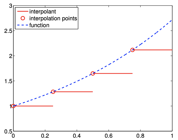
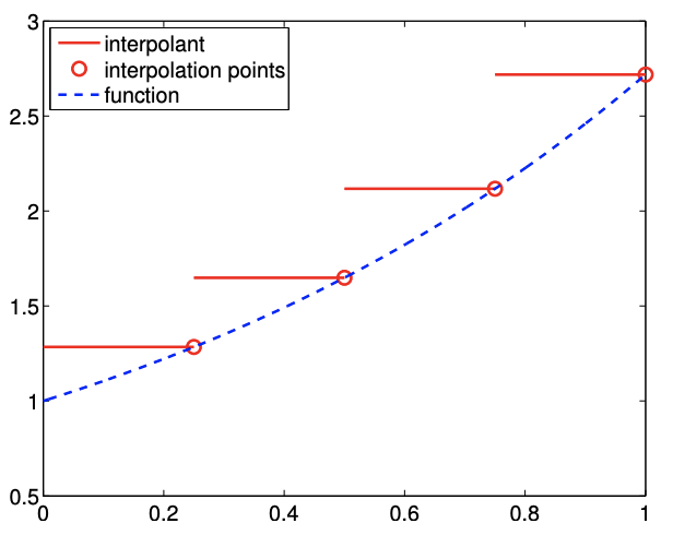
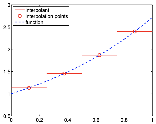
The first example we consider uses a piecewise-constant polynomial to approximate the function \(f\). Because a constant polynomial is parameterized by a single value, this scheme requires one interpolation point per interval, meaning \(M=1\). On each segment \(S_{i}=\left[x_{i}, x_{i+1}\right]\), we choose the left endpoint as our interpolation point, i.e. \[\bar{x}^{1}=x_{i}\] As shown in Figure \(2.3\), we can also easily associate the segmentation points, \(x_{i}\), with the global function evaluation points, \(\tilde{x}_{i}\), i.e. \[\tilde{x}_{i}=x_{i}, \quad i=1, \ldots, N-1\] Extending the left-endpoint value to the rest of the segment, we obtain the interpolant of the form \[(\mathcal{I} f)(x)=f\left(\bar{x}^{1}\right)=f\left(\tilde{x}_{i}\right)=f\left(x_{i}\right), \quad \forall x \in S_{i}\] Figure 2.4(a) shows the interpolation scheme applied to \(f(x)=\exp (x)\) over \([0,1]\) with \(N=\) 5. Because \(f^{\prime}>0\) over each interval, the interpolant \(\mathcal{I} f\) always underestimate the value of \(f\). Conversely, if \(f^{\prime}<0\) over an interval, the interpolant overestimates the values of \(f\) in the interval. The interpolant is exact over the interval if \(f\) is constant.

If \(f^{\prime}\) exists, the error in the interpolant is bounded by \[e_{i} \leq h \cdot \max _{x \in S_{i}}\left|f^{\prime}(x)\right|\] \({ }^{1}\) for the interpolants considered in this chapter

Figure 2.3: The relationship between the discretization, a local segment, and the function evaluation points for a piecewise-constant, left-endpoint interpolant.

(a) interpolant

(b) error

Figure 2.4: Piecewise-constant, left-endpoint interpolant.

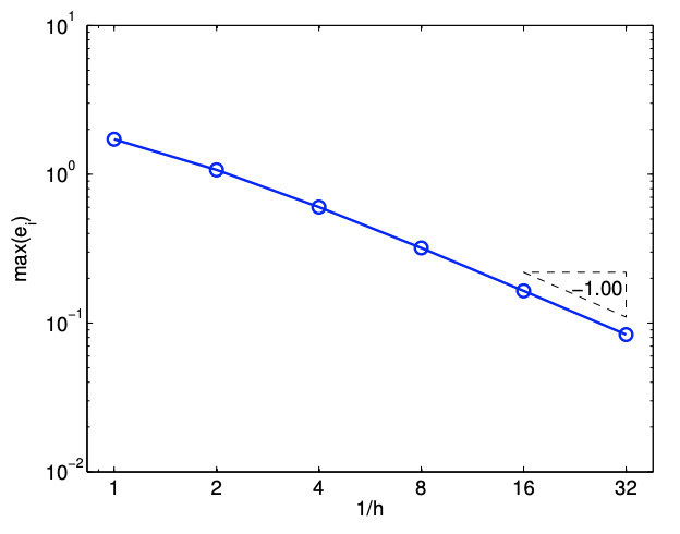
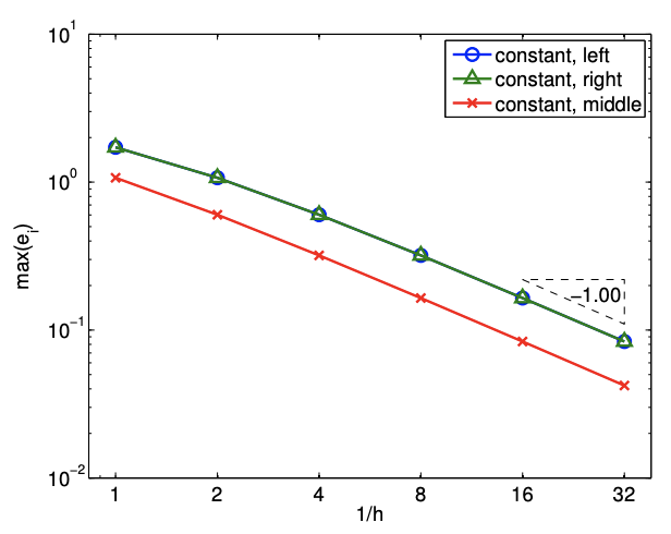
Since \(e_{i}=\mathcal{O}(h)\) and the error scales as the first power of \(h\), the scheme is said to be first-order accurate. The convergence behavior of the interpolant applied to the exponential function is shown in Figure 2.4(b), where the maximum value of the interpolation error, \(e_{\max }=\max _{i} e_{i}\), is plotted as a function of the number of intervals, \(1 / h\).

We pause to review two related concepts that characterize asymptotic behavior of a sequence: the big- \(\mathcal{O}\) notation \((\mathcal{O}(\cdot))\) and the asymptotic notation \((\sim)\). Say that \(Q\) and \(z\) are scalar quantities (real numbers) and \(q\) is a function of \(z\). Using the big- \(\mathcal{O}\) notation, when we say that \(Q\) is \(\mathcal{O}(q(z)\) ) as \(z\) tends to, say, zero (or infinity), we mean that there exist constants \(C_{1}\) and \(z^{*}\) such that \(|Q|<C_{1}|q(z)|, \forall z<z^{*}\) (or \(\forall z>z^{*}\) ). On the other hand, using the asymptotic notation, when we say that \(Q \sim C_{2} q(z)\) as \(z\) tends to some limit, we mean that there exist a constant \(C_{2}\) (not necessary equal to \(\left.C_{1}\right)\) such that \(Q /\left(C_{2} q(z)\right)\) tends to unity as \(z\) tends to the limit. We shall use these notations in two cases in particular: (i) when \(z\) is \(\delta\), a discretization parameter ( \(h\) in our example above) - which tends to zero; (ii) when \(z\) is \(K\), an integer related to the number of degrees of freedom that define a problem ( \(N\) in our example above) - which tends to infinity. Note we need not worry about small effects with the \(\mathcal{O}\) (or the asymptotic) notation: for \(K\) tends to infinity, for example, \(\mathcal{O}(K)=\mathcal{O}(K-1)=\mathcal{O}(K+\sqrt{K})\). Finally, we note that the expression \(Q=\mathcal{O}(1)\) means that \(Q\) effectively does not depend on some (implicit, or "understood") parameter, \(z .^{2}\)

If \(f(x)\) is linear, then the error bound can be shown using a direct argument. Let \(f(x)=\overline{m x}+b\). The difference between the function and the interpolant over \(S_{i}\) is \[f(x)-(\mathcal{I} f)(x)=[m x-b]-\left[m \bar{x}^{1}-b\right]=m \cdot\left(x-\bar{x}^{1}\right) .\] Recalling the local error is the maximum difference in the function and interpolant and noting that \(S_{i}=\left[x_{i}, x_{i+1}\right]=\left[\bar{x}^{1}, \bar{x}^{1}+h\right]\), we obtain \[e_{i}=\max _{x \in S_{i}}|f(x)-(\mathcal{I} f)(x)|=\max _{x \in S_{i}}\left|m \cdot\left(x-\bar{x}^{1}\right)\right|=|m| \cdot \max _{x \in\left[\bar{x}^{1}, \bar{x}^{1}+h\right]}\left|x-\bar{x}^{1}\right|=|m| \cdot h .\] Finally, recalling that \(m=f^{\prime}(x)\) for the linear function, we have \(e_{i}=\left|f^{\prime}(x)\right| \cdot h\). Now, let us prove the error bound for a general \(f\).

Proof

The proof follows from the definition of the interpolant and the fundamental theorem of calculus, i.e. \[f(x)-(\mathcal{I} f)(x)=f(x)-f\left(\bar{x}^{1}\right) \quad \text { (by definition of }(\mathcal{I} f) \text { ) }\] \[\begin{aligned} & =\int_{\bar{z} 1}^{x} f^{\prime}(\xi) d \xi \quad \text { (fundamental theorem of calculus) } \\ & \leq \int_{\bar{x}^{1}}^{x}\left|f^{\prime}(\xi)\right| d \xi \\ & \leq \max _{x \in\left[\bar{x}^{1}, x\right]}\left|f^{\prime}(x)\right|\left|\int_{\bar{x}^{1}}^{x} d \xi\right| \end{aligned}\] (Hölder’s inequality) \[\begin{aligned} & \leq \max _{x \in S_{i}}\left|f^{\prime}(x)\right| \cdot h, \quad \forall x \in S_{i}=\left[\bar{x}^{1}, \bar{x}^{1}+h\right] . \end{aligned}\] Substitution of the expression into the definition of the error yields \[e_{i} \equiv \max _{x \in S_{i}}|f(x)-(\mathcal{I} f)(x)| \leq \max _{x \in S_{i}}\left|f^{\prime}(x)\right| \cdot h .\] \({ }^{2}\) The engineering notation \(Q=\mathcal{O}\left(10^{3}\right)\) is somewhat different and really just means that the number is roughly \(10^{3} .\)

\({ }^{2}\) The engineering notation \(Q=\mathcal{O}\left(10^{3}\right)\) is somewhat different and really just means that the number is roughly \(10^{3} .\)

(a) interpolant

(b) error

Figure 2.5: Piecewise-constant, left-endpoint interpolant for a non-smooth function.

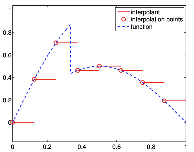
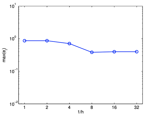
It is important to note that the proof relies on the smoothness of \(f\). In fact, if \(f\) is discontinuous and \(f^{\prime}\) does not exist, then \(e_{i}\) can be \(\mathcal{O}(1)\). In other words, the interpolant does not converge to the function (in the sense of maximum error), even if the \(h\) is refined. To demonstrate this, let us consider a function \[f(x)=\left\{\begin{array}{ll} \sin (\pi x), & x \leq \frac{1}{3} \\ \frac{1}{2} \sin (\pi x), & x>\frac{1}{3} \end{array},\right.\] which is discontinuous at \(x=1 / 3\). The result of applying the piecewise constant, left-endpoint rule to the function is shown in Figure 2.5(a). We note that the solution on the third segment is not approximated well due to the presence of the discontinuity. More importantly, the convergence plot, Figure 2.5(b), confirms that the maximum interpolation error does not converge even if \(h\) is refined. This reduction in the convergence rate for non-smooth functions is not unique to this particular interpolation rule; all interpolation rules suffer from this problem. Thus, we must be careful when we interpolate a non-smooth function.

Finally, we comment on the distinction between the "best fit" (in some norm, or metric) and the interpolant. The best fit in the "max" or "sup" norm of a constant function \(c_{i}\) to \(f(x)\) over \(S_{i}\) minimizes \(\left|c_{i}-f(x)\right|\) over \(S_{i}\) and will typically be different and perforce better (in the chosen norm) than the interpolant. However, the determination of \(c_{i}\) in principle requires knowledge of \(f(x)\) at (almost) all points in \(S_{i}\) whereas the interpolant only requires knowledge of \(f(x)\) at one point - hence much more useful. We discuss this further in Section 2.1.1.

Let us more formally define some of the key concepts visited in the first example. While we introduce the following concepts in the context of analyzing the interpolation schemes, the concepts apply more generally to analyzing various numerical schemes.

• Accuracy relates how well the numerical scheme (finite-dimensional) approximates the continuous system (infinite-dimensional). In the context of interpolation, the accuracy tells how well the interpolant \(\mathcal{I} f\) approximates \(f\) and is measured by the interpolation error, \(e_{\max }\). - Convergence is the property that the error vanishes as the discretization is refined, i.e.

\[e_{\max } \rightarrow 0 \quad \text { as } \quad h \rightarrow 0 .\] A convergent scheme can achieve any desired accuracy (error) in infinite prediction arithmetics by choosing \(h\) sufficiently small. The piecewise-constant, left-endpoint interpolant is a convergent scheme, because \(e_{\max }=\mathcal{O}(h)\), and \(e_{\max } \rightarrow 0\) as \(h \rightarrow 0\).

• Convergence rate is the power \(p\) such that

\[e_{\max } \leq C h^{p} \quad \text { as } \quad h \rightarrow 0,\] where \(C\) is a constant independent of \(h\). The scheme is first-order accurate for \(p=1\), secondorder accurate for \(p=2\), and so on. The piecewise-constant, left-endpoint interpolant is first-order accurate because \(e_{\max }=C h^{1}\). Note here \(p\) is fixed and the convergence (with number of intervals) is thus algebraic.

Note that typically as \(h \rightarrow 0\) we obtain not a bound but in fact asymptotic behavior: \(e_{\max } \sim\) \(C h^{p}\) or equivalently, \(e_{\max } /\left(C h^{p}\right) \rightarrow 1\), as \(h \rightarrow 0\). Taking the logarithm of \(e_{\max } \sim C h^{p}\), we obtain \(\ln \left(e_{\max }\right) \sim \ln C+p \ln h\). Thus, a \(\log -\log\) plot is a convenient means of finding \(p\) empirically.

• Resolution is the characteristic length \(h_{\text {crit }}\) for any particular problem (described by \(f\) ) for which we see the asymptotic convergence rate for \(h \leq h_{\text {crit. }}\). Convergence plot in Figure \(2.4\) (b) shows that the piecewise-constant, left-endpoint interpolant achieves the asymptotic convergence rate of 1 with respect to \(h\) for \(h \leq 1 / 2\); note that the slope from \(h=1\) to \(h=1 / 2\) is lower than unity. Thus, \(h_{\text {crit }}\) for the interpolation scheme applied to \(f(x)=\exp (x)\) is approximately \(1 / 2\).
• Computational cost or operation count is the number of floating point operations (FLOPs \({ }^{3}\) ) to compute \(I_{h}\). As \(h \rightarrow 0\), the number of FLOPs approaches \(\infty\). The scaling of the computation cost with the size of the problem is referred to as computational complexity. The actual runtime of computation is a function of the computational cost and the hardware. The cost of constructing the piecewise-constant, left end point interpolant is proportional to the number of segments. Thus, the cost scales linearly with \(N\), and the scheme is said to have linear complexity.
• Memory or storage is the number of floating point numbers that must be stored at any point during execution.

We note that the above properties characterize a scheme in infinite precision representation and arithmetic. Precision is related to machine precision, floating point number truncation, rounding and arithmetic errors, etc, all of which are absent in infinite-precision arithmetics.

We also note that there are two conflicting demands; the accuracy of the scheme increases with decreasing \(h\) (assuming the scheme is convergent), but the computational cost increases with decreasing \(h\). Intuitively, this always happen because the dimension of the discrete approximation must be increased to better approximate the continuous system. However, some schemes produce lower error for the same computational cost than other schemes. The performance of a numerical scheme is assessed in terms of the accuracy it delivers for a given computational cost.

We will now visit several other interpolation schemes and characterize the schemes using the above properties.

\({ }^{3}\) Not to be confused with the FLOPS (floating point operations per second), which is often used to measure the performance of a computational hardware.

Figure 2.6: Piecewise-constant, right-endpoint interpolant.

Example 2.1.2 piecewise-constant, right end point

This interpolant also uses a piecewise-constant polynomial to approximate the function \(f\), and thus requires one interpolation point per interval, i.e., \(M=1\). This time, the interpolation point is at the right endpoint, instead of the left endpoint, resulting in \[\bar{x}^{1}=x_{i+1}, \quad(\mathcal{I} f)(x)=f\left(\bar{x}^{1}\right)=f\left(x_{i+1}\right), \quad \forall x \in S_{i}=\left[x_{i}, x_{i+1}\right] .\] The global function evaluation points, \(\tilde{x}_{i}\), are related to segmentation points, \(x_{i}\), by \[\tilde{x}_{i}=x_{i+1}, \quad i=1, \ldots, N-1 .\] Figure \(2.6\) shows the interpolation applied to the exponential function.

If \(f^{\prime}\) exists, the error in the interpolant is bounded by \[e_{i} \leq h \cdot \max _{x \in S_{i}}\left|f^{\prime}(x)\right|,\] and thus the scheme is first-order accurate. The proof is similar to that of the piecewise-constant, right-endpoint interpolant.

Example 2.1.3 piecewise-constant, midpoint

This interpolant uses a piecewise-constant polynomial to approximate the function \(f\), but uses the midpoint of the segment, \(S_{i}=\left[x_{i}, x_{i+1}\right]\), as the interpolation point, i.e. \[\bar{x}^{1}=\frac{1}{2}\left(x_{i}+x_{i+1}\right) .\] Denoting the (global) function evaluation point associated with segment \(S_{i}\) as \(\tilde{x}_{i}\), we have \[\tilde{x}_{i}=\frac{1}{2}\left(x_{i}+x_{i+1}\right), \quad i=1, \ldots, N-1,\] as illustrated in Figure 2.7. Note that the segmentation points \(x_{i}\) do not correspond to the function evaluation points \(\tilde{x}_{i}\) unlike in the previous two interpolants. This choice of interpolation point results in the interpolant \[(\mathcal{I} f)(x)=f\left(\bar{x}^{1}\right)=f\left(\tilde{x}_{i}\right)=f\left(\frac{1}{2}\left(x_{i}+x_{i+1}\right)\right), \quad x \in S_{i} .\]

Figure 2.7: The relationship between the discretization, a local segment, and the function evaluation points for a piecewise-constant, midpoint interpolant.

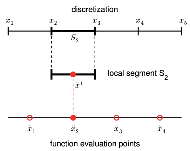
Figure 2.8(a) shows the interpolant for the exponential function. In the context of table lookup, this interpolant naturally arises if a value is approximated from a table of data choosing the nearest data point.

The error of the interpolant is bounded by \[e_{i} \leq \frac{h}{2} \cdot \max _{x \in S_{i}}\left|f^{\prime}(x)\right|,\] where the factor of half comes from the fact that any function evaluation point is less than \(h / 2\) distance away from one of the interpolation points. Figure \(2.8(\mathrm{a})\) shows that the midpoint interpolant achieves lower error than the left- or right-endpoint interpolant. However, the error still scales linearly with \(h\), and thus the midpoint interpolant is first-order accurate.

For a linear function \(f(x)=m x+b\), the sharp error bound can be obtained from a direct argument. The difference between the function and its midpoint interpolant is \[f(x)-(\mathcal{I} f)(x)=[m x+b]-\left[m \bar{x}^{1}+b\right]=m \cdot\left(x-\bar{x}^{1}\right) .\] The difference vanishes at the midpoint, and increases linearly with the distance from the midpoint. Thus, the difference is maximized at either of the endpoints. Noting that the segment can be expressed as \(S_{i}=\left[x_{i}, x_{i+1}\right]=\left[\bar{x}^{1}-\frac{h}{2}, \bar{x}^{1}+\frac{h}{2}\right]\), the maximum error is given by \[\begin{aligned} e_{i} & \equiv \max _{x \in S_{i}}(f(x)-(\mathcal{I} f)(x))=\max _{x \in\left[\bar{x}^{1}-\frac{h}{2}, \bar{x}^{1}+\frac{h}{2}\right]}\left|m \cdot\left(x-\bar{x}^{1}\right)\right| \\ &=\left|m \cdot\left(x-\bar{x}^{1}\right)\right|_{x=\bar{x}^{1} \pm h / 2}=|m| \cdot \frac{h}{2} . \end{aligned}\] Recalling \(m=f^{\prime}(x)\) for the linear function, we have \(e_{i}=\left|f^{\prime}(x)\right| h / 2\). A sharp proof for a general \(f\) follows essentially that for the piecewise-constant, left-endpoint rule.

(a) interpolant

(b) error

Figure 2.8: Piecewise-constant, mid point interpolant.

Proof

The proof follows from the fundamental theorem of calculus, \[\begin{aligned} f(x)-(\mathcal{I} f)(x) &=f(x)-f\left(\bar{x}^{1}\right)=\int_{\bar{x}^{1}}^{x} f^{\prime}(\xi) d \xi \leq \int_{\bar{x}^{1}}^{x}\left|f^{\prime}(\xi)\right| d \xi \leq \max _{x \in\left[\bar{x}^{1}, x\right]}\left|f^{\prime}(x)\right|\left|\int_{\bar{x}^{1}}^{x} d \xi\right| \\ & \leq \max _{x \in\left[\bar{x}^{1}-\frac{h}{2}, \bar{x}^{1}+\frac{h}{2}\right]}^{\left|f^{\prime}(x)\right| \cdot \frac{h}{2}, \quad \forall x \in S_{i}=\left[\bar{x}^{1}-\frac{h}{2}, \bar{x}^{1}+\frac{h}{2}\right]} \end{aligned}\] Thus, we have \[e_{i}=\max _{x \in S_{i}}|f(x)-(\mathcal{I} f)(x)| \leq \max _{x \in S_{i}}\left|f^{\prime}(x)\right| \cdot \frac{h}{2}\]

Example 2.1.4 piecewise-linear

The three examples we have considered so far used piecewise-constant functions to interpolate the function of interest, resulting in the interpolants that are first-order accurate. In order to improve the quality of interpolation, we consider a second-order accurate interpolant in this example. To achieve this, we choose a piecewise-linear function (i.e., first-degree polynomials) to approximate the function behavior. Because a linear function has two coefficients, we must choose two interpolation points per segment to uniquely define the interpolant, i.e., \(M=2\). In particular, for segment \(S_{i}=\left[x_{i}, x_{i+1}\right]\), we choose its endpoints, \(x_{i}\) and \(x_{i+1}\), as the interpolation points, i.e. \[\bar{x}^{1}=x_{i} \quad \text { and } \quad \bar{x}^{2}=x_{i+1}\] The (global) function evaluation points and the segmentation points are trivially related by \[\tilde{x}_{i}=x_{i}, \quad i=1, \ldots, N,\]

Figure 2.9: The relationship between the discretization, a local segment, and the function evaluation points for a linear interpolant.

as illustrated in Figure \(2.9\).

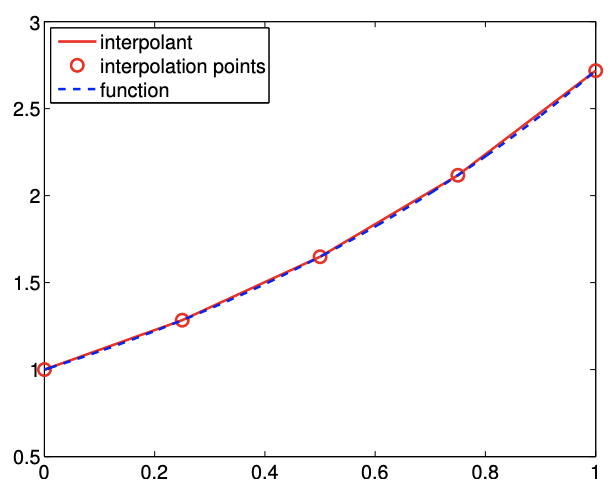
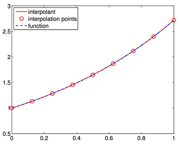
The resulting interpolant, defined using the local coordinate, is of the form \[(\mathcal{I} f)(x)=f\left(\bar{x}^{1}\right)+\left(\frac{f\left(\bar{x}^{2}\right)-f\left(\bar{x}^{1}\right)}{h}\right)\left(x-\bar{x}^{1}\right), \quad \forall x \in S_{i},\] or, in the global coordinate, is expressed as \[(\mathcal{I} f)(x)=f\left(x_{i}\right)+\left(\frac{f\left(x_{i+1}\right)-f\left(x_{i}\right)}{h_{i}}\right)\left(x-x_{i}\right), \quad \forall x \in S_{i} .\] Figure \(2.10(\) a \()\) shows the linear interpolant applied to \(f(x)=\exp (x)\) over \([0,1]\) with \(N=5\). Note that this interpolant is continuous across the segment endpoints, because each piecewise-linear function matches the true function values at its endpoints. This is in contrast to the piecewiseconstant interpolants considered in the previous three examples, which were discontinuous across the segment endpoints in general.

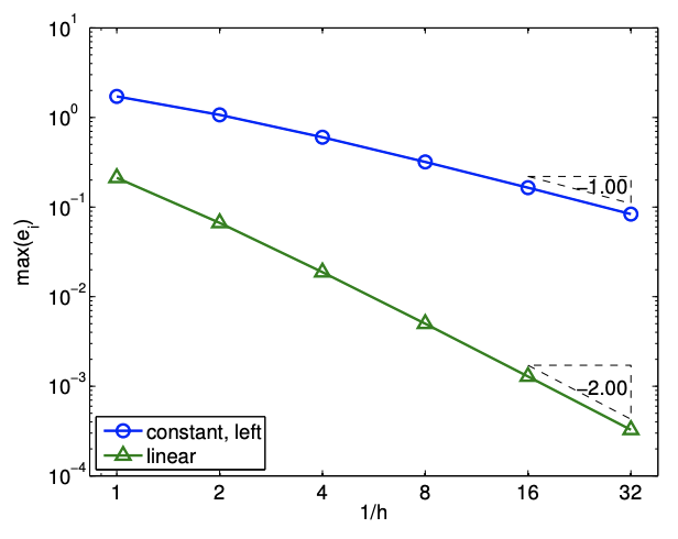
If \(f^{\prime \prime}\) exists, the error of the linear interpolant is bounded by \[e_{i} \leq \frac{h^{2}}{8} \cdot \max _{x \in S_{i}}\left|f^{\prime \prime}(x)\right|\] The error of the linear interpolant converges quadratically with the interval length, \(h\). Because the error scales with \(h^{2}\), the method is said to be second-order accurate. Figure \(2.10\) (b) shows that the linear interpolant is significantly more accurate than the piecewise-linear interpolant for the exponential function. This trend is generally true for sufficient smooth functions. More importantly, the higher-order convergence means that the linear interpolant approaches the true function at a faster rate than the piecewise-constant interpolant as the segment length decreases.

Let us provide a sketch of the proof. First, noting that \(f(x)-(\mathcal{I} f)(x)\) vanishes at the endpoints, we express our error as \[f(x)-(\mathcal{I} f)(x)=\int_{\bar{x}^{1}}^{x}(f-\mathcal{I} f)^{\prime}(t) d t\] Next, by the Mean Value Theorem (MVT), we have a point \(x^{*} \in S_{i}=\left[\bar{x}^{1}, \bar{x}^{2}\right]\) such that \(f^{\prime}\left(x^{*}\right)-\) \((\mathcal{I} f)^{\prime}\left(x^{*}\right)=0\). Note the MVT - for a continuously differentiable function \(f\) there exists an

(a) interpolant

(b) error

Figure 2.10: Piecewise-linear interpolant.

\(x^{*} \in\left[\bar{x}^{1}, \bar{x}^{2}\right]\) such that \(f^{\prime}\left(x^{*}\right)=\left(f\left(\bar{x}^{2}\right)-f\left(\bar{x}^{1}\right)\right) / h-\) follows from Rolle’s Theorem. Rolle’s Theorem states that, for a continuously differentiable function \(g\) that vanishes at \(\bar{x}^{1}\) and \(\bar{x}^{2}\), there exists a point \(x^{*}\) for which \(g^{\prime}\left(x^{*}\right)=0\). To derive the MVT we take \(g(x)=f(x)-\mathcal{I} f(x)\) for \(\mathcal{I} f\) given by Eq. (2.1). Applying the fundamental theorem of calculus again, the error can be expressed as \[\begin{aligned} f(x)-(\mathcal{I} f)(x) &=\int_{\bar{x}^{1}}^{x}(f-\mathcal{I} f)^{\prime}(t) d t=\int_{\bar{x}^{1}}^{x} \int_{x^{*}}^{t}(f-\mathcal{I} f)^{\prime \prime}(s) d s d t=\int_{\bar{x}^{1}}^{x} \int_{x^{*}}^{t} f^{\prime \prime}(s) d s d t \\ & \leq \max _{x \in S_{i}}\left|f^{\prime \prime}(x)\right| \int_{\bar{x}^{1}}^{x} \int_{x^{*}}^{t} d s d t \leq \frac{h^{2}}{2} \cdot \max _{x \in S_{i}}\left|f^{\prime \prime}(x)\right| \end{aligned}\] This simple sketch shows that the interpolation error is dependent on the second derivative of \(f\) and quadratically varies with the segment length \(h\); however, the constant is not sharp. A sharp proof is provided below.

Proof

Our objective is to obtain a bound for \(|f(\hat{x})-\mathcal{I} f(\hat{x})|\) for an arbitrary \(\hat{x} \in S_{i}\). If \(\hat{x}\) is the one of the endpoints, the interpolation error vanishes trivially; thus, we assume that \(\hat{x}\) is not one of the endpoints. The proof follows from a construction of a particular quadratic interpolant and the application of the Rolle’s theorem. First let us form the quadratic interpolant, \(q(x)\), of the form \[q(x) \equiv(\mathcal{I} f)(x)+\lambda w(x) \quad \text { with } \quad w(x)=\left(x-\bar{x}^{1}\right)\left(x-\bar{x}^{2}\right) .\] Since \((\mathcal{I} f)\) matches \(f\) at \(\bar{x}^{1}\) and \(\bar{x}^{2}\) and \(q\left(\bar{x}^{1}\right)=q\left(\bar{x}^{2}\right)=0, q(x)\) matches \(f\) at \(\bar{x}^{1}\) and \(\bar{x}^{2}\). We select \(\lambda\) such that \(q\) matches \(f\) at \(\hat{x}\), i.e. \[q(\hat{x})=(\mathcal{I} f)(\hat{x})+\lambda w(\hat{x})=f(\hat{x}) \Rightarrow \lambda=\frac{f(\hat{x})-(\mathcal{I} f)(\hat{x})}{w(\hat{x})}\] The interpolation error of the quadratic interpolant is given by \[\phi(x)=f(x)-q(x)\] Because \(q\) is the quadratic interpolant of \(f\) defined by the interpolation points \(\bar{x}^{1}, \bar{x}^{2}\), and \(\hat{x}, \phi\) has three zeros in \(S_{i}\). By Rolle’s theorem, \(\phi^{\prime}\) has two zeros in \(S_{i}\). Again, by Rolle’s theorem, \(\phi^{\prime \prime}\) has one zero in \(S_{i}\). Let this zero be denoted by \(\xi\), i.e., \(\phi^{\prime \prime}(\xi)=0\). Evaluation of \(\phi^{\prime \prime}(\xi)\) yields \[0=\phi^{\prime \prime}(\xi)=f^{\prime \prime}(\xi)-q^{\prime \prime}(\xi)=f^{\prime \prime}(\xi)-(\mathcal{I} f)^{\prime \prime}(\xi)-\lambda w^{\prime \prime}(\xi)=f^{\prime \prime}(\xi)-2 \lambda \quad \Rightarrow \quad \lambda=\frac{1}{2} f^{\prime \prime}(\xi) .\] Evaluating \(\phi(\hat{x})\), we obtain \[\begin{aligned} 0 &=\phi(\hat{x})=f(\hat{x})-(\mathcal{I} f)(\hat{x})-\frac{1}{2} f^{\prime \prime}(\xi) w(\hat{x}) \\ f(\hat{x})-(\mathcal{I} f)(\hat{x}) &=\frac{1}{2} f^{\prime \prime}(\xi)\left(\hat{x}-\bar{x}^{1}\right)\left(\hat{x}-\bar{x}^{2}\right) . \end{aligned}\] The function is maximized for \(\hat{x}^{*}=\left(\bar{x}^{1}+\bar{x}^{2}\right) / 2\), which yields \[f(\hat{x})-(\mathcal{I} f)(\hat{x}) \leq \frac{1}{8} f^{\prime \prime}(\xi)\left(\bar{x}^{2}-\bar{x}^{1}\right)^{2}=\frac{1}{8} h^{2} f^{\prime \prime}(\xi), \quad \forall \hat{x} \in\left[\bar{x}^{1}, \bar{x}^{2}\right]\] Since \(\xi \in S_{i}\), it follows that, \[e_{i}=\max _{x \in S_{i}}|f(x)-(\mathcal{I} f)(x)| \leq \frac{1}{8} h^{2} f^{\prime \prime}(\xi) \leq \frac{1}{8} h^{2} \max _{x \in S_{i}}\left|f^{\prime \prime}(x)\right| .\]

Example 2.1.5 piecewise-quadratic

Motivated by the higher accuracy provided by the second-order accurate, piecewise-linear interpolants, we now consider using a piecewise-quadratic polynomial to construct an interpolant. Because a quadratic function is characterized by three parameters, we require three interpolation points per segment \((M=3)\). For segment \(S_{i}=\left[x_{i}, x_{i+1}\right]\), a natural choice are the two endpoints and the midpoint, i.e. \[\bar{x}^{1}=x_{i}, \quad \bar{x}^{2}=\frac{1}{2}\left(x_{i}+x_{i+1}\right), \quad \text { and } \quad \bar{x}^{3}=x_{i+1} .\] To construct the interpolant, we first construct Lagrange basis polynomial of the form \[\phi_{1}(x)=\frac{\left(x-\bar{x}^{2}\right)\left(x-\bar{x}^{3}\right)}{\left(\bar{x}^{1}-\bar{x}^{2}\right)\left(\bar{x}^{1}-\bar{x}^{3}\right)}, \quad \phi_{2}(x)=\frac{\left(x-\bar{x}^{1}\right)\left(x-\bar{x}^{3}\right)}{\left(\bar{x}^{2}-\bar{x}^{1}\right)\left(\bar{x}^{2}-\bar{x}^{3}\right)}, \quad \text { and } \quad \phi_{3}(x)=\frac{\left(x-\bar{x}^{1}\right)\left(x-\bar{x}^{2}\right)}{\left(\bar{x}^{3}-\bar{x}^{1}\right)\left(\bar{x}^{3}-\bar{x}^{2}\right)} .\] By construction, \(\phi_{1}\) takes the value of 1 at \(\bar{x}^{1}\) and vanishes at \(\bar{x}^{2}\) and \(\bar{x}^{3}\). More generally, the Lagrange basis has the property \[\phi_{m}\left(\bar{x}^{n}\right)=\left\{\begin{array}{ll} 1, & n=m \\ 0, & n \neq m \end{array} .\right.\] Using these basis functions, we can construct the quadratic interpolant as \[(\mathcal{I} f)(x)=f\left(\bar{x}^{1}\right) \phi_{1}(x)+f\left(\bar{x}^{2}\right) \phi_{2}(x)+f\left(\bar{x}^{3}\right) \phi_{3}(x), \quad \forall x \in S_{i} .\]

(a) interpolant

(b) error

Figure 2.11: Piecewise-quadratic interpolant.

We can easily confirm that the quadratic function goes through the interpolation points, \(\left(\bar{x}^{m}, f\left(\bar{x}^{m}\right)\right)\), \(m=1,2,3\), using the property of the Lagrange basis. Figure 2.11(a) shows the interpolant for the exponential function.

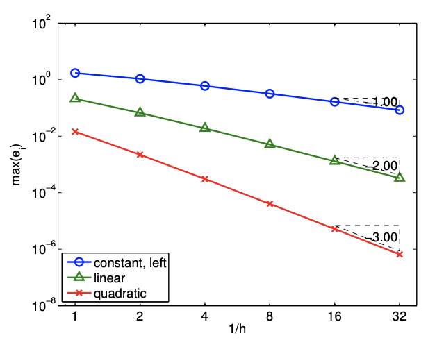
If \(f^{\prime \prime \prime}\) exists, the error of the quadratic interpolant is bounded by \[e_{i} \leq \frac{h^{3}}{72 \sqrt{3}} \max _{x \in S_{i}} f^{\prime \prime \prime}(x) .\] The error converges as the cubic power of \(h\), meaning the scheme is third-order accurate. Figure \(2.11\) (b) confirms the higher-order convergence of the piecewise-quadratic interpolant.

Proof

The proof is an extension of that for the linear interpolant. First, we form a cubic interpolant of the form \[q(x) \equiv(\mathcal{I} f)(x)+\lambda w(x) \quad \text { with } \quad w(x)=\left(x-\bar{x}^{1}\right)\left(x-\bar{x}^{2}\right)\left(x-\bar{x}^{3}\right) .\] We select \(\lambda\) such that \(q\) matches \(f\) at \(\hat{x}\). The interpolation error function, \[\phi(x)=f(x)-q(x),\] has four zeros in \(S_{i}\), specifically \(\bar{x}^{1}, \bar{x}^{2}, \bar{x}^{3}\), and \(\hat{x}\). By repeatedly applying the Rolle’s theorem three times, we note that \(\phi^{\prime \prime \prime}(x)\) has one zero in \(S_{i}\). Let us denote this zero by \(\xi\), i.e., \(\phi^{\prime \prime \prime}(\xi)=0\). This implies that \[\phi^{\prime \prime \prime}(\xi)=f^{\prime \prime \prime}(\xi)-(c I f)^{\prime \prime \prime}(\xi)-\lambda w^{\prime \prime \prime}(\xi)=f^{\prime \prime \prime}(\xi)-6 \lambda=0 \quad \Rightarrow \quad \lambda=\frac{1}{6} f^{\prime \prime \prime}(\xi) .\] Rearranging the expression for \(\phi(\hat{x})\), we obtain \[f(\hat{x})-(\mathcal{I} f)(\hat{x})=\frac{1}{6} f^{\prime \prime \prime}(\xi) w(\hat{x}) .\]

(a) interpolant

(b) error

Figure 2.12: Piecewise-quadratic interpolant for a non-smooth function.

The maximum value that \(w\) takes over \(S_{i}\) is \(h^{3} /(12 \sqrt{3})\). Combined with the fact \(f^{\prime \prime \prime}(\xi) \leq\) \(\max _{x \in S_{i}} f^{\prime \prime \prime}(x)\), we obtain the error bound \[e_{i}=\max _{x \in S_{i}}|f(x)-(\mathcal{I} f)(x)| \leq \frac{h^{3}}{72 \sqrt{3}} \max _{x \in S_{i}} f^{\prime \prime \prime}(x) .\] Note that the extension of this proof to higher-order interpolants is straight forward. In general, a piecewise \(p^{\text {th }}\)-degree polynomial interpolant exhibits \(p+1\) order convergence.

The procedure for constructing the Lagrange polynomials extends to arbitrary degree polynomials. Thus, in principle, we can construct an arbitrarily high-order interpolant by increasing the number of interpolation points. While the higher-order interpolation yielded a lower interpolation error for the smooth function considered, a few cautions are in order.

First, higher-order interpolants are more susceptible to modeling errors. If the underlying data is noisy, the "overfitting" of the noisy data can lead to inaccurate interpolant. This will be discussed in more details in Unit III on regression.

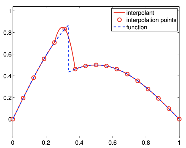
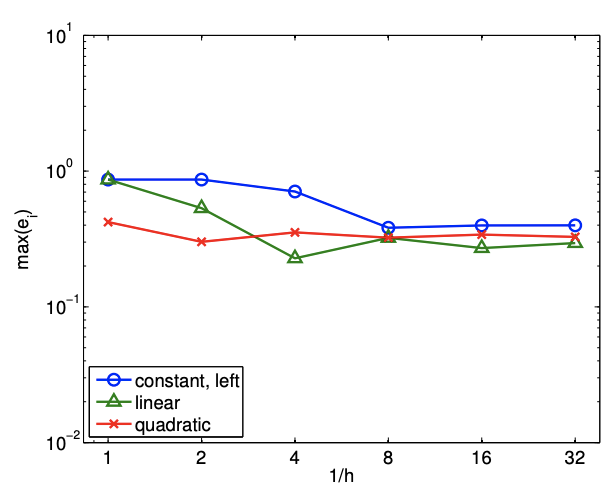
Second, higher-order interpolants are also typically not advantageous for non-smooth functions. To see this, we revisit the simple discontinuous function, \[f(x)=\left\{\begin{array}{ll} \sin (\pi x), & x \leq \frac{1}{3} \\ \frac{1}{2} \sin (\pi x), & x>\frac{1}{3} \end{array} .\right.\] The result of applying the piecewise-quadratic interpolation rule to the function is shown in Figure \(2.12(\mathrm{a})\). The quadratic interpolant closely matches the underlying function in the smooth region. However, in the third segment, which contains the discontinuity, the interpolant differs considerably from the underlying function. Similar to the piecewise-constant interpolation of the function, we again commit \(\mathcal{O}(1)\) error measured in the maximum difference. Figure \(2.12\) (b) confirms that the higher-order interpolants do not perform any better than the piecewise-constant interpolant in the presence of discontinuity. Formally, we can show that the maximum-error convergence of any interpolation scheme can be no better than \(h^{r}\), where \(r\) is the highest-order derivative that is defined everywhere in the domain. In the presence of a discontinuity, \(r=0\), and we observe \(\mathcal{O}\left(h^{r}\right)=\mathcal{O}(1)\) convergence (i.e., no convergence).

Third, for a very high-order polynomials, the interpolation points must be chosen carefully to achieve a good result. In particular, the uniform distribution suffers from the behavior known as Runge’s phenomenon, where the interpolant exhibits excessive oscillation even if the underlying function is smooth. The spurious oscillation can be minimized by clustering the interpolation points near the segment endpoints, e.g., Chebyshev nodes.

Advanced Material

Interpolation: Polynomials of Degree \(n\)

We will study in more details how the choice of interpolation points affect the quality of a polynomial interpolant. For convenience, let us denote the space of \(n^{\mathrm{th}}\)-degree polynomials on segment \(S\) by \(\mathcal{P}_{n}(S)\). For consistency, we will denote \(n^{\text {th }}\)-degree polynomial interpolant of \(f\), which is defined by \(n+1\) interpolation points \(\left\{\bar{x}^{m}\right\}_{m=1}^{n+1}\), by \(\mathcal{I}_{n} f\). We will compare the quality of the interpolant with the "best" \(n+1\) degree polynomial. We will define "best" in the infinity norm, i.e., the best polynomial \(v^{*} \in \mathcal{P}_{n}(S)\) satisfies \[\max _{x \in S}\left|f(x)-v^{*}(x)\right| \leq \max _{x \in S}|f(x)-v(x)|, \quad \forall v \in \mathcal{P}_{n}(x) .\] In some sense, the polynomial \(v^{*}\) fits the function \(f\) as closely as possible. Then, the quality of a \(n^{\text {th }}\)-degree interpolant can be assessed by measuring how close it is to \(v^{*}\). More precisely, we quantify its quality by comparing the maximum error of the interpolant with that of the best polynomial, i.e. \[\max _{x \in S}|f(x)-(\mathcal{I} f)(x)| \leq\left(1+\Lambda\left(\left\{\bar{x}^{m}\right\}_{m=1}^{n+1}\right)\right) \max _{x \in S}\left|f(x)-v^{*}(x)\right|,\] where the constant \(\Lambda\) is called the Lebesgue constant. Clearly, a smaller Lebesgue constant implies smaller error, so higher the quality of the interpolant. At the same time, \(\Lambda \geq 0\) because the maximum error in the interpolant cannot be better than that of the "best" function, which by definition minimizes the maximum error. In fact, the Lebesgue constant is given by \[\Lambda\left(\left\{\bar{x}^{m}\right\}_{m=1}^{n+1}\right)=\max _{x \in S} \sum_{m=1}^{n+1}\left|\phi_{m}(x)\right|,\] where \(\phi_{m}, m=1, \ldots, n+1\), are the Lagrange bases functions defined by the nodes \(\left\{\bar{x}^{m}\right\}_{m=1}^{n+1}\).

Proof. We first express the interpolation error in the infinity norm as the sum of two contributions \[\begin{aligned} \max _{x \in S}|f(x)-(\mathcal{I} f)(x)| & \leq \max _{x \in S}\left|f(x)-v^{*}(x)+v^{*}(x)-(\mathcal{I} f)(x)\right| \\ & \leq \max _{x \in S}\left|f(x)-v^{*}(x)\right|+\max _{x \in S}\left|v^{*}(x)-(\mathcal{I} f)(x)\right| . \end{aligned}\] Noting that the functions in the second term are polynomial, we express them in terms of the Lagrange basis \(\phi_{m}, m=1, \ldots, n\), \[\begin{aligned} \max _{x \in S}\left|v^{*}(x)-(\mathcal{I} f)(x)\right| &=\max _{x \in S}\left|\sum_{m=1}^{n+1}\left(v^{*}\left(\bar{x}^{m}\right)-(\mathcal{I} f)\left(\bar{x}^{m}\right)\right) \phi_{m}(x)\right| \\ & \leq \max _{x \in S}\left|\max _{m=1, \ldots, n+1}\right| v^{*}\left(\bar{x}^{m}\right)-(\mathcal{I} f)\left(\bar{x}^{m}\right)\left|\cdot \sum_{m=1}^{n+1}\right| \phi_{m}(x)|| \\ &=\max _{m=1, \ldots, n+1}\left|v^{*}\left(\bar{x}^{m}\right)-(\mathcal{I} f)\left(\bar{x}^{m}\right)\right| \cdot \max _{x \in S} \sum_{m=1}^{n+1}\left|\phi_{m}(x)\right| . \end{aligned}\] Because \(\mathcal{I} f\) is an interpolant, we have \(f\left(\bar{x}^{m}\right)=(\mathcal{I} f)\left(\bar{x}^{m}\right), m=1, \ldots, n+1\). Moreover, we recognize that the second term is the expression for Lebesgue constant. Thus, we have \[\begin{aligned} \max _{x \in S}\left|v^{*}(x)-(\mathcal{I} f)(x)\right| & \leq \max _{m=1, \ldots, n+1}\left|v^{*}\left(\bar{x}^{m}\right)-f\left(\bar{x}^{m}\right)\right| \cdot \Lambda \\ & \leq \max _{x \in S}\left|v^{*}(x)-f(x)\right| \Lambda . \end{aligned}\] where the last inequality follows from recognizing \(\bar{x}^{m} \in S, m=1, \ldots, n+1\). Thus, the interpolation error in the maximum norm is bounded by \[\begin{aligned} \max _{x \in S}|f(x)-(\mathcal{I} f)(x)| & \leq \max _{x \in S}\left|v^{*}(x)-f(x)\right|+\max _{x \in S}\left|v^{*}(x)-f(x)\right| \Lambda \\ & \leq(1+\Lambda) \max _{x \in S}\left|v^{*}(x)-f(x)\right|, \end{aligned}\] which is the desired result.

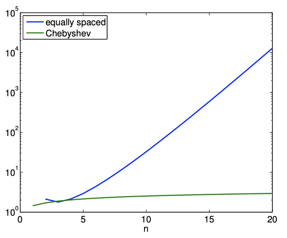
In the previous section, we noted that equally spaced points can produce unstable interpolants for a large \(n\). In fact, the Lebesgue constant for the equally spaced node distribution varies as \[\Lambda \sim \frac{2^{n}}{e n \log (n)},\] i.e., the Lebesgue constant increases exponentially with \(n\). Thus, increasing \(n\) does not necessary results in a smaller interpolation error.

A more stable interpolant can be formed using the Chebyshev node distribution. The node distribution is given (on \([-1,1])\) by \[\bar{x}^{m}=\cos \left(\frac{2 m-1}{2(n+1)} \pi\right), \quad m=1, \ldots, n+1 .\] Note that the nodes are clustered toward the endpoints. The Lebesgue constant for Chebyshev node distribution is \[\Lambda=1+\frac{2}{\pi} \log (n+1),\] i.e., the constant grows much more slowly. The variation in the Lebesgue constant for the equallyspaced and Chebyshev node distributions are shown in Figure \(\underline{2.13}\).

Figure 2.13: The approximate Lebesgue constants for equally-spaced and Chebyshev node distributions.

(a) equally spaced

(b) Chebyshev distribution

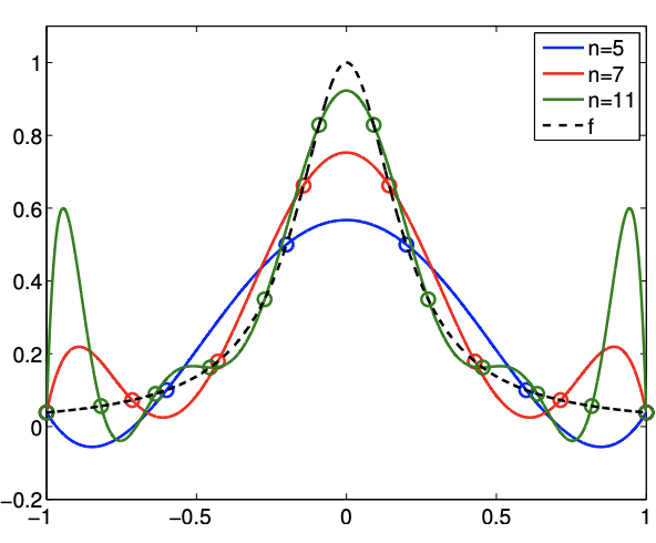
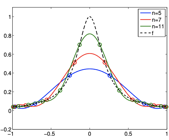
Figure 2.14: High-order interpolants for \(f=1 /\left(x+25 x^{2}\right)\) over \([-1,1]\).

Example 2.1.6 Runge’s phenomenon

To demonstrate the instability of interpolants based on equally-spaced nodes, let us consider interpolation of \[f(x)=\frac{1}{1+25 x^{2}}\] The resulting interpolants for \(p=5,7\), and 11 are shown in Figure 2.14. Note that equally-spaced nodes produce spurious oscillation near the end of the intervals. On the other hand, the clustering of the nodes toward the endpoints allow the Chebyshev node distribution to control the error in the region.

Advanced Material

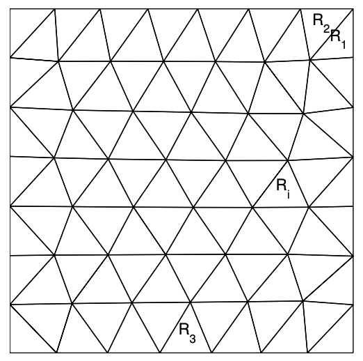
(a) mesh

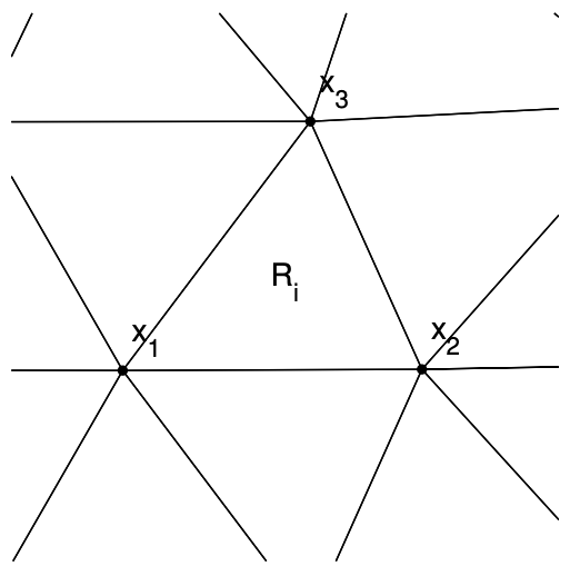
(b) triangle \(R_{i}\)

Figure 2.15: Triangulation of a 2-D domain.