2.2.1: Discrete Random Variables

Probability Mass Functions

In this chapter, we develop mathematical tools for describing and analyzing random experiments, experiments whose outcome cannot be determined with certainty. A coin flip and a roll of a die are classical examples of such experiments. The outcome of a random experiment is described by a random variable \(X\) that takes on a finite number of values, \[x_{1}, \ldots, x_{J} \text {, }\] where \(J\) is the number of values that \(X\) takes. To fully characterize the behavior of the random variable, we assign a probability to each of these events, i.e. \[X=x_{j}, \quad \text { with probability } p_{j}, \quad j=1, \ldots, J .\] The same information can be expressed in terms of the probability mass function (pmf), or discrete density function, \(f_{X}\), that assigns a probability to each possible outcome \[f_{X}\left(x_{j}\right)=p_{j}, \quad j=1, \ldots, J .\] In order for \(f_{X}\) to be a valid probability density function, \(\left\{p_{j}\right\}\) must satisfy \[\begin{aligned} &0 \leq p_{j} \leq 1, \quad j=1, \ldots, J, \\ &\sum_{j=1}^{J} p_{j}=1 \end{aligned}\] The first condition requires that the probability of each event be non-negative and be less than or equal to unity. The second condition states that \(\left\{x_{1}, \ldots, x_{J}\right\}\) includes the set of all possible values that \(X\) can take, and that the sum of the probabilities of the outcome is unity. The second condition follows from the fact that events \(x_{i}, i=1, \ldots, J\), are mutually exclusive and collectively exhaustive. Mutually exclusive means that \(X\) cannot take on two different values of the \(x_{i}\) ’s in any given experiment. Collectively exhaustive means that \(X\) must take on one of the \(J\) possible values in any given experiment. Note that for the same random phenomenon, we can choose many different outcomes; i.e. we can characterize the phenomenon in many different ways. For example, \(x_{j}=j\) could simply be a label for the \(j\)-th outcome; or \(x_{j}\) could be a numerical value related to some attribute of the phenomenon. For instance, in the case of flipping a coin, we could associate a numerical value of 1 with heads and 0 with tails. Of course, if we wish, we could instead associate a numerical value of 0 with heads and 1 with tails to describe the same experiment. We will see examples of many different random variables in this unit. The key point is that the association of a numerical value to an outcome allows us to introduce meaningful quantitative characterizations of the random phenomenon - which is of course very important in the engineering context.

Let us define a few notions useful for characterizing the behavior of the random variable. The expectation of \(X, E[X]\), is defined as \[E[X]=\sum_{j=1}^{J} x_{j} p_{j} .\] The expectation of \(X\) is also called the mean. We denote the mean by \(\mu\) or \(\mu_{X}\), with the second notation emphasizing that it is the mean of \(X\). Note that the mean is a weighted average of the values taken by \(X\), where each weight is specified according to the respective probability. This is analogous to the concept of moment in mechanics, where the distances are provided by \(x_{j}\) and the weights are provided by \(p_{j}\); for this reason, the mean is also called the first moment. The mean corresponds to the centroid in mechanics.

Note that, in frequentist terms, the mean may be expressed as the sum of values taken by \(X\) over a large number of realizations divided by the number of realizations, i.e. \[(\text { Mean })=\lim _{\text {(# Realizations) } \rightarrow \infty} \frac{1}{\text { (# Realizations) }} \sum_{j=1}^{J} x_{j} \cdot\left(\# \text { Occurrences of } x_{j}\right) .\] Recalling that the probability of a given event is defined as \[p_{j}=\lim _{(\# \text { Realizations) } \rightarrow \infty} \frac{\left(\# \text { Occurrences of } x_{j}\right)}{\text { (# Realizations) }},\] we observe that \[E[X]=\sum_{j=1}^{J} x_{j} p_{j}\] which is consistent with the definition provided in Eq. (9.1). Let us provide a simple gambling scenario to clarity this frequentist interpretation of the mean. Here, we consider a "game of chance" that has \(J\) outcomes with corresponding probabilities \(p_{j}, j=1, \ldots, J\); we denote by \(x_{j}\) the (net) pay-off for outcome \(j\). Then, in \(n_{\text {plays }}\) plays of the game, our (net) income would be \[\sum_{j=1}^{J} x_{j} \cdot \text { (# Occurrences of } x_{j} \text { ), }\] which in the limit of large \(n_{\text {plays }}\left(=\right.\) # Realizations) yields \(n_{\text {plays }} \cdot E[X]\). In other words, the mean \(E[X]\) is the expected pay-off per play of the game, which agrees with our intuitive sense of the mean. The variance, or the second moment about the mean, measures the spread of the values about the mean and is defined by \[\operatorname{Var}[X] \equiv E\left[(X-\mu)^{2}\right]=\sum_{j=1}^{J}\left(x_{j}-\mu\right)^{2} p_{j}\] We denote the variance as \(\sigma^{2}\). The variance can also be expressed as \[\begin{aligned} \operatorname{Var}[X] &=E\left[(X-\mu)^{2}\right]=\sum_{j=1}^{J}\left(x_{j}-\mu\right)^{2} p_{j}=\sum_{j=1}^{J}\left(x_{j}^{2}-2 x_{j} \mu+\mu^{2}\right) p_{j} \\ &=\underbrace{\sum_{j=1}^{J} x_{j}^{2} p_{j}}_{E\left[X^{2}\right]}-2 \mu \underbrace{\sum_{j=1}^{J} x_{j} p_{j}}_{\mu}+\mu^{\mu^{2} \sum_{j=1}^{J} p_{j}}=E\left[X^{2}\right]-\mu^{2} . \end{aligned}\] Note that the variance has the unit of \(X\) squared. Another useful measure of the expected spread of the random variable is standard deviation, \(\sigma\), which is defined by \[\sigma=\sqrt{\operatorname{Var}[X]} .\] We typically expect departures from the mean of many standard deviations to be rare. This is particularly the case for random variables with large range, i.e. \(J\) large. (For discrete random variables with small \(J\), this spread interpretation is sometimes not obvious simply because the range of \(X\) is small.) In case of the aforementioned "game of chance" gambling scenario, the standard deviation measures the likely (or expected) deviation in the pay-off from the expectation (i.e. the mean). Thus, the standard deviation can be related in various ways to risk; high standard deviation implies a high-risk case with high probability of large payoff (or loss).

The mean and variance (or standard deviation) provide a convenient way of characterizing the behavior of a probability mass function. In some cases the mean and variance (or even the mean alone) can serve as parameters which completely determine a particular mass function. In many other cases, these two properties may not suffice to completely determine the distribution but can still serve as useful measures from which to make further deductions.

Let us consider a few examples of discrete random variables.

Example 9.1.1 rolling a die

As the first example, let us apply the aforementioned framework to rolling of a die. The random variable \(X\) describes the outcome of rolling a (fair) six-sided die. It takes on one of six possible values, \(1,2, \ldots, 6\). These events are mutually exclusive, because a die cannot take on two different values at the same time. Also, the events are exhaustive because the die must take on one of the six values after each roll. Thus, the random variable \(X\) takes on one of the six possible values, \[x_{1}=1, x_{2}=2, \ldots, x_{6}=6 .\] A fair die has the equal probability of producing one of the six outcomes, i.e. \[X=x_{j}=j, \quad \text { with probability } \frac{1}{6}, \quad j=1, \ldots, 6,\] or, in terms of the probability mass function, \[f_{X}(x)=\frac{1}{6}, \quad x=1, \ldots, 6 .\]

(a) realization

(b) pmf

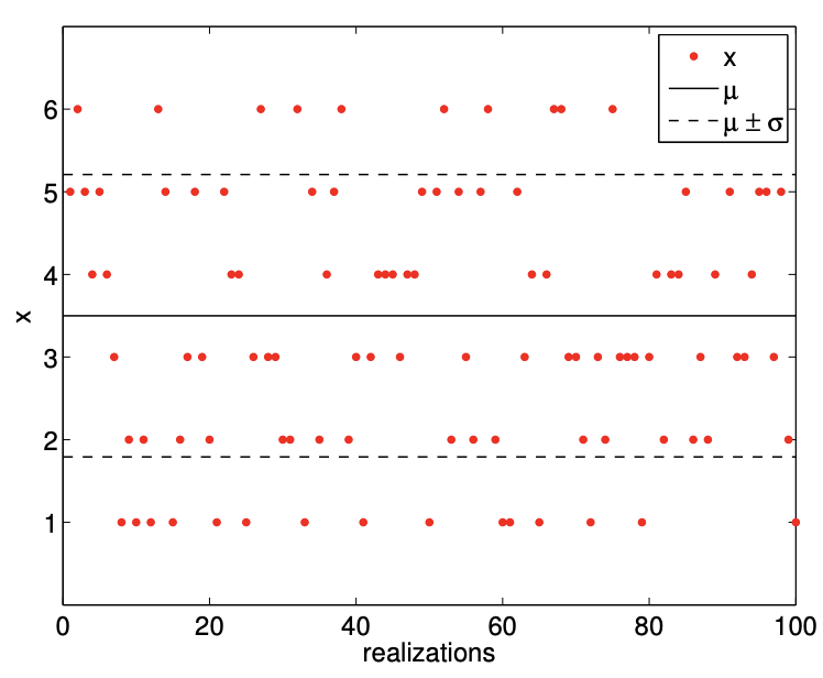
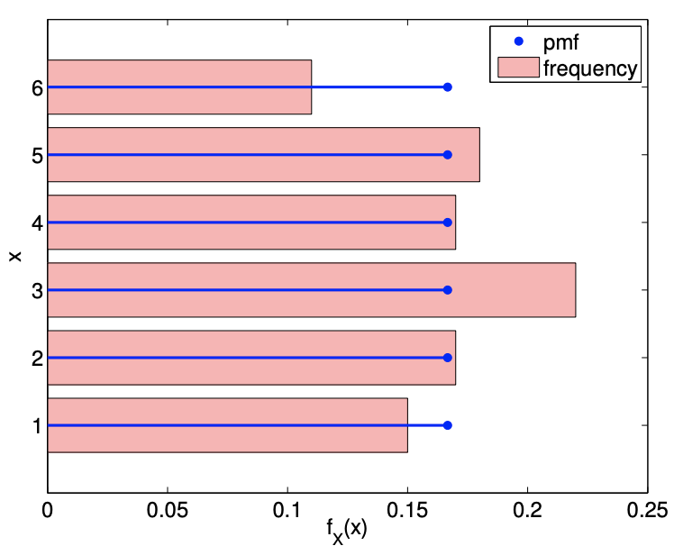
Figure 9.1: Illustration of the values taken by a fair six-sided die and the probability mass function.

An example of outcome of a hundred die rolls is shown in Figure 9.1(a). The die always takes on one of the six values, and there is no obvious inclination toward one value or the other. This is consistent with the fact that any one of the six values is equally likely. (In practice, we would like to think of Figure 9.1(a) as observed outcomes of actual die rolls, i.e. data, though for convenience here we use synthetic data through random number generation (which we shall discuss subsequently).)

Figure 9.1(b) shows the probability mass function, \(f_{X}\), of the six equally likely events. The figure also shows the relative frequency of each event - which is defined as the number of occurrences of the event normalized by the total number of samples (which is 100 for this case) - as a histogram. Even for a relatively small sample size of 100 , the histogram roughly matches the probability mass function. We can imagine that as the number of samples increases, the relative frequency of each event gets closer and closer to its value of probability mass function.

Conversely, if we have an experiment with an unknown probability distribution, we could infer its probability distribution through a large number of trials. Namely, we can construct a histogram, like the one shown in Figure 9.1(b), and then construct a probability mass function that fits the histogram. This procedure is consistent with the frequentist interpretation of probability: the probability of an event is the relative frequency of its occurrence in a large number of samples. The inference of the underlying probability distribution from a limited amount of data (i.e. a small sample) is an important problem often encountered in engineering practice.

Let us now characterize the probability mass function in terms of the mean and variance. The mean of the distribution is \[\mu=E[X]=\sum_{j=1}^{6} x_{j} p_{j}=\sum_{j=1}^{6} j \cdot \frac{1}{6}=\frac{7}{2}\] The variance of the distribution is \[\sigma^{2}=\operatorname{Var}[X]=E\left[X^{2}\right]-\mu^{2} \sum_{j=1}^{6} x_{j}^{2} p_{j}-\mu^{2}=\sum_{j=1}^{6} j^{2} \cdot \frac{1}{6}-\left(\frac{7}{2}\right)^{2}=\frac{91}{6}-\frac{49}{4}=\frac{35}{12} \approx 2.9167,\] and the standard deviation is \[\sigma=\sqrt{\operatorname{Var}[X]}=\sqrt{\frac{35}{12}} \approx 1.7078\]

Example 9.1.2 (discrete) uniform distribution

The outcome of rolling a (fair) die is a special case of a more general distribution, called the (discrete) uniform distribution. The uniform distribution is characterized by each event having the equal probability. It is described by two integer parameters, \(a\) and \(b\), which assign the lower and upper bounds of the sample space, respectively. The distribution takes on \(J=b-a+1\) values. For the six-sided die, we have \(a=1, b=6\), and \(J=b-a+1=6\). In general, we have \[\begin{aligned} x_{j} &=a+j-1, \quad j=1, \ldots, J, \\ f^{\text {disc.uniform }}(x) &=\frac{1}{J} . \end{aligned}\] The mean and variance of a (discrete) uniform distribution are given by \[\mu=\frac{a+b}{2} \text { and } \quad \sigma^{2}=\frac{J^{2}-1}{12} .\] We can easily verify that the expressions are consistent with the die rolling case with \(a=1, b=6\), and \(J=6\), which result in \(\mu=7 / 2\) and \(\sigma^{2}=35 / 12\).

Proof

The mean follows from \[\begin{aligned} \mu &=E[X]=E[X-(a-1)+(a-1)]=E[X-(a-1)]+a-1 \\ &=\sum_{j=1}^{J}\left(x_{j}-(a-1)\right) p_{j}+a-1=\sum_{j=1}^{J} j \frac{1}{J}+a-1=\frac{1}{J} \frac{J(J+1)}{2}+a-1 \\ &=\frac{b-a+1+1}{2}+a-1=\frac{b+a}{2} . \end{aligned}\] The variance follows from \[\begin{aligned} \sigma^{2} &=\operatorname{Var}[X]=E\left[(X-E[X])^{2}\right]=E\left[((X-(a-1))-E[X-(a-1)])^{2}\right] \\ &=E\left[(X-(a-1))^{2}\right]-E[X-(a-1)]^{2} \\ &=\sum_{j=1}^{J}\left(x_{j}-(a-1)\right)^{2} p_{j}-\left[\sum_{j=1}^{J}\left(x_{j}-(a-1)\right) p_{j}\right]^{2} \\ &=\sum_{j=1}^{J} j^{2} \frac{1}{J}-\left[\sum_{j=1}^{J} j p_{j}\right]^{2}=\frac{1}{J} \frac{J(J+1)(2 J+1)}{6}-\left[\frac{1}{J} \frac{J(J+1)}{2}\right]^{2} \\ &=\frac{J^{2}-1}{12}=\frac{(b-a+1)^{2}-1}{12} . \end{aligned}\]

Example 9.1.3 Bernoulli distribution (a coin flip)

Consider a classical random experiment of flipping a coin. The outcome of a coin flip is either a head or a tail, and each outcome is equally likely assuming the coin is fair (i.e. unbiased). Without loss of generality, we can associate the value of 1 (success) with head and the value of 0 (failure) with tail. In fact, the coin flip is an example of a Bernoulli experiment, whose outcome takes on either 0 or 1 .

Specifically, a Bernoulli random variable, \(X\), takes on two values, 0 and 1 , i.e. \(J=2\), and \[x_{1}=0 \quad \text { and } \quad x_{2}=1 .\] The probability mass function is parametrized by a single parameter, \(\theta \in[0,1]\), and is given by \[f_{X_{\theta}}(x)=f^{\text {Bernoulli }}(x ; \theta) \equiv\left\{\begin{array}{l} 1-\theta, \quad x=0 \\ \theta, \quad x=1 \end{array}\right.\] In other words, \(\theta\) is the probability that the random variable \(X_{\theta}\) takes on the value of 1 . Flipping of a fair coin is a particular case of a Bernoulli experiment with \(\theta=1 / 2\). The \(\theta=1 / 2\) case is also a special case of the discrete uniform distribution with \(a=0\) and \(b=1\), which results in \(J=2\). Note that, in our notation, \(f_{X_{\theta}}\) is the probability mass function associated with a particular random variable \(X_{\theta}\), whereas \(f^{\text {Bernoulli }}(\cdot ; \theta)\) is a family of distributions that describe Bernoulli random variables. For notational simplicity, we will not explicitly state the parameter dependence of \(X_{\theta}\) on \(\theta\) from hereon, unless the explicit clarification is necessary, i.e. we will simply use \(X\) for the random variable and \(f_{X}\) for its probability mass function. (Also note that what we call a random variable is of course our choice, and, in the subsequent sections, we often use variable \(B\), instead of \(X\), for a Bernoulli random variable.)

Examples of the values taken by Bernoulli random variables with \(\theta=1 / 2\) and \(\theta=1 / 4\) are shown in Figure 9.2. As expected, with \(\theta=1 / 2\), the random variable takes on the value of 0 and 1 roughly equal number of times. On the other hand, \(\theta=1 / 4\) results in the random variable taking on 0 more frequently than 1 .

The probability mass functions, shown in Figure \(9.2\), reflect the fact that \(\theta=1 / 4\) results in \(X\) taking on 0 three times more frequently than 1 . Even with just 100 samples, the relative frequency histograms captures the difference in the frequency of the events for \(\theta=1 / 2\) and \(\theta=1 / 4\). In fact, even if we did not know the underlying pmf - characterized by \(\theta\) in this case - we can infer from the sampled data that the second case has a lower probability of success (i.e. \(x=1\) ) than the first case. In the subsequent chapters, we will formalize this notion of inferring the underlying distribution from samples and present a method for performing the task.

The mean and variance of the Bernoulli distribution are given by \[E[X]=\theta \quad \text { and } \quad \operatorname{Var}[X]=\theta(1-\theta) .\] Note that lower \(\theta\) results in a lower mean, because the distribution is more likely to take on the value of 0 than 1 . Note also that the variance is small for either \(\theta \rightarrow 0\) or \(\theta \rightarrow 1\) as in these cases we are almost sure to get one or the other outcome. But note that (say) \(\sigma / E(X)\) scales as \(1 / \sqrt{(\theta)}\) (recall \(\sigma\) is the standard deviation) and hence the relative variation in \(X\) becomes more pronounced for small \(\theta\) : this will have important consequences in our ability to predict rare events.

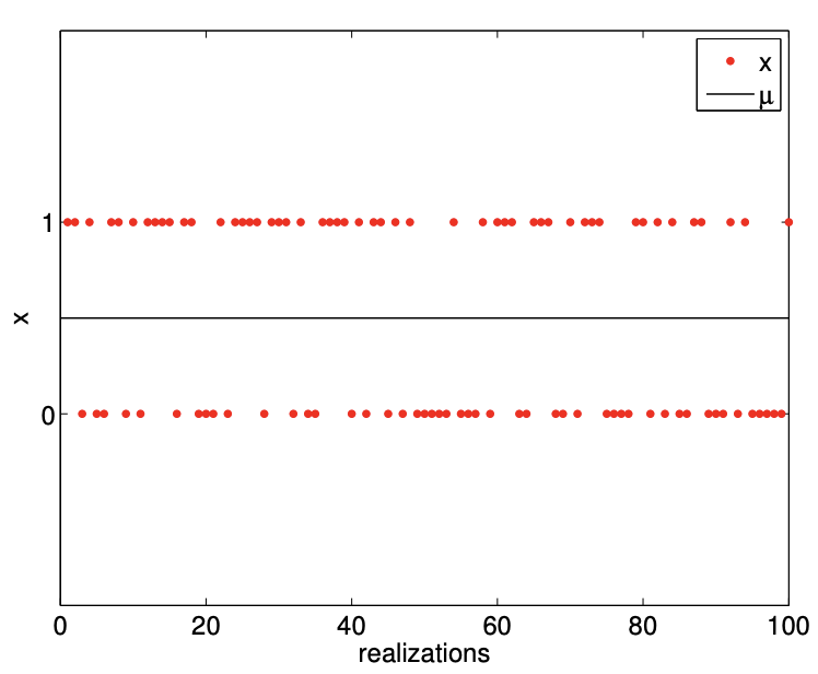
(a) realization, \(\theta=1 / 2\)

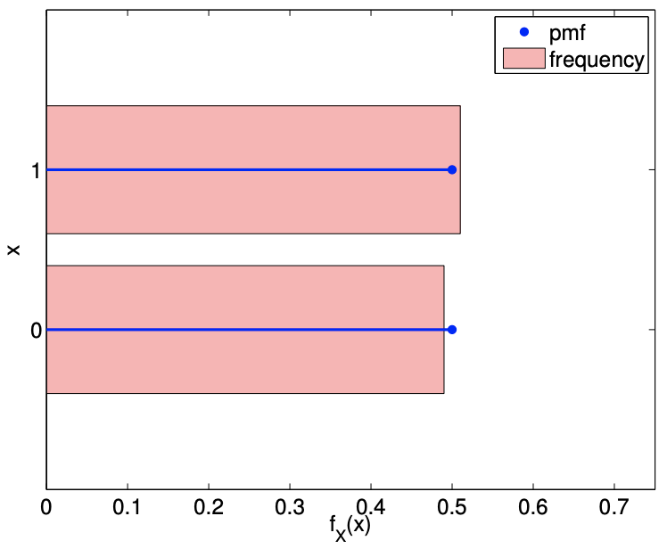
(b) \(\mathrm{pmf}, \theta=1 / 2\)

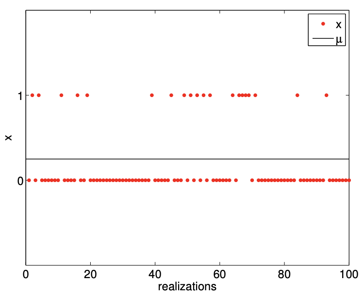
(c) realization, \(\theta=1 / 4\)

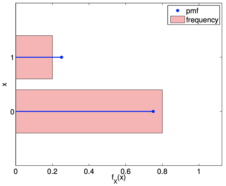
(d) \(\operatorname{pmf}, \theta=1 / 4\)

Figure 9.2: Illustration of the values taken by Bernoulli random variables and the probability mass functions.

Proof

Proof of the mean and variance follows directly from the definitions. The mean is given by \[\mu=E[X]=\sum_{j=1}^{J} x_{j} p_{j}=0 \cdot(1-\theta)+1 \cdot \theta=\theta .\] The variance is given by \[\operatorname{Var}[X]=E\left[(X-\mu)^{2}\right]=\sum_{j=1}^{J}\left(x_{j}-\mu\right)^{2} p_{j}=(0-\theta)^{2} \cdot(1-\theta)+(1-\theta)^{2} \cdot \theta=\theta(1-\theta) .\]

Before concluding this subsection, let us briefly discuss the concept of "events." We can define an event of \(A\) or \(B\) as the random variable \(X\) taking on one of some set mutually exclusive outcomes \(x_{j}\) in either the set \(A\) or the set \(B\). Then, we have \[P(A \text { or } B)=P(A \cup B)=P(A)+P(B)-P(A \cap B) .\] That is, probability of event \(A\) or \(B\) taking place is equal to double counting the outcomes \(x_{j}\) in both \(A\) and \(B\) and then subtracting out the outcomes in both \(A\) and \(B\) to correct for this double counting. Note that, if \(A\) and \(B\) are mutually exclusive, we have \(A \cap B=\emptyset\) and \(P(A \cap B)=0\). Thus the probability of \(A\) or \(B\) is \[P(A \text { or } B)=P(A)+P(B), \quad(A \text { and } B \text { mutually exclusive }) .\] This agrees with our intuition that if \(A\) and \(B\) are mutually exclusive, we would not double count outcomes and thus would not need to correct for it.

Transformation

Random variables, just like deterministic variables, can be transformed by a function. For example, if \(X\) is a random variable and \(g\) is a function, then a transformation \[Y=g(X)\] produces another random variable \(Y\). Recall that we described the behavior of \(X\) that takes on one of \(J\) values by \[X=x_{j} \text { with probability } p_{j}, \quad j=1, \ldots, J .\] The associated probability mass function was \(f_{X}\left(x_{j}\right)=p_{j}, j=1, \ldots, J\). The transformation \(Y=g(X)\) yields the set of outcomes \(y_{j}, j=1, \ldots, J\), where each \(y_{j}\) results from applying \(g\) to \(x_{j}\), i.e. \[y_{j}=g\left(x_{j}\right), \quad j=1, \ldots, J .\] Thus, \(Y\) can be described by \[Y=y_{j}=g\left(x_{j}\right) \quad \text { with probability } p_{j}, \quad j=1, \ldots, J .\] We can write the probability mass function of \(Y\) as \[f_{Y}\left(y_{j}\right)=f_{Y}\left(g\left(x_{j}\right)\right)=p_{j} \quad j=1, \ldots, J .\] We can express the mean of the transformed variable in a few different ways: \[E[Y]=\sum_{j=1}^{J} y_{j} f_{Y}\left(y_{j}\right)=\sum_{j=1}^{J} y_{j} p_{j}=\sum_{j=1}^{J} g\left(x_{j}\right) f_{X}\left(x_{j}\right) .\] The first expression expresses the mean in terms of \(Y\) only, whereas the final expression expresses \(E[Y]\) in terms of \(X\) and \(g\) without making a direct reference to \(Y\).

Let us consider a specific example.

Example 9.1.4 from rolling a die to flipping a coin

Let us say that we want to create a random experiment with equal probability of success and failure (e.g. deciding who goes first in a football game), but all you have is a die instead of a coin. One way to create a Bernoulli random experiment is to roll the die, and assign "success" if an odd number is rolled and assign "failure" if an even number is rolled.

Let us write out the process more formally. We start with a (discrete) uniform random variable \(X\) that takes on \[x_{j}=j, \quad j=1, \ldots, 6,\] with probability \(p_{j}=1 / 6, j=1, \ldots, 6\). Equivalently, the probability density function for \(X\) is \[f_{X}(x)=\frac{1}{6}, \quad x=1,2, \ldots, 6 .\] Consider a function \[g(x)= \begin{cases}0, & x \in\{1,3,5\} \\ 1, & x \in\{2,4,6\}\end{cases}\] Let us consider a random variable \(Y=g(X)\). Mapping the outcomes of \(X, x_{1}, \ldots, x_{6}\), to \(y_{1}^{\prime}, \ldots, y_{6}^{\prime}\), we have \[\begin{aligned} &y_{1}^{\prime}=g\left(x_{1}\right)=g(1)=0, \\ &y_{2}^{\prime}=g\left(x_{2}\right)=g(2)=1, \\ &y_{3}^{\prime}=g\left(x_{3}\right)=g(3)=0, \\ &y_{4}^{\prime}=g\left(x_{4}\right)=g(4)=1, \\ &y_{5}^{\prime}=g\left(x_{5}\right)=g(5)=0, \\ &y_{6}^{\prime}=g\left(x_{6}\right)=g(6)=1 . \end{aligned}\] We could thus describe the transformed variable \(Y\) as \[Y=y_{j}^{\prime} \quad \text { with probability } p_{j}=1 / 6, \quad j=1, \ldots, 6 .\] However, because \(y_{1}^{\prime}=y_{3}^{\prime}=y_{5}^{\prime}\) and \(y_{2}^{\prime}=y_{4}^{\prime}=y_{6}^{\prime}\), we can simplify the expression. Without loss of generality, let us set \[y_{1}=y_{1}^{\prime}=y_{3}^{\prime}=y_{5}^{\prime}=0 \quad \text { and } \quad y_{2}=y_{2}^{\prime}=y_{4}^{\prime}=y_{6}^{\prime}=1 .\]

Figure 9.3: Transformation of \(X\) associated with a die roll to a Bernoulli random variable \(Y\).

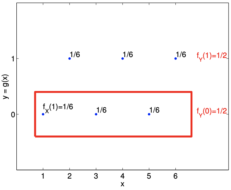
We now combine the frequentist interpretation of probability with the fact that \(x_{1}, \ldots, x_{6}\) are mutually exclusive. Recall that to a frequentist, \(P\left(Y=y_{1}=0\right)\) is the probability that \(Y\) takes on 0 in a large number of trials. In order for \(Y\) to take on 0 , we must have \(x=1,3\), or 5 . Because \(X\) taking on 1, 3, and 5 are mutually exclusive events (e.g. \(X\) cannot take on 1 and 3 at the same time), the number of occurrences of \(y=0\) is equal to the sum of the number of occurrences of \(x=1, x=3\), and \(x=5\). Thus, the relative frequency of \(Y\) taking on \(0-\) or its probability - is equal to the sum of the relative frequencies of \(X\) taking on 1,3 , or 5 . Mathematically, \[P\left(Y=y_{1}=0\right)=P(X=1)+P(X=3)+P(X=5)=\frac{1}{6}+\frac{1}{6}+\frac{1}{6}=\frac{1}{2} .\] Similarly, because \(X\) taking on 2,4 , and 6 are mutually exclusive events, \[P\left(Y=y_{2}=1\right)=P(X=2)+P(X=4)+P(X=6)=\frac{1}{6}+\frac{1}{6}+\frac{1}{6}=\frac{1}{2} .\] Thus, we have \[Y= \begin{cases}0, & \text { with probability } 1 / 2 \\ 1, & \text { with probability } 1 / 2,\end{cases}\] or, in terms of the probability density function, \[f_{Y}(y)=\frac{1}{2}, \quad y=0,1 .\] Note that we have transformed the uniform random variable \(X\) by the function \(g\) to create a Bernoulli random variable \(Y\). We emphasize that the mutually exclusive property of \(x_{1}, \ldots, x_{6}\) is the key that enables the simple summation of probability of the events. In essence, (say), \(y=0\) obtains if \(x=1\) OR if \(x=3\) OR if \(x=5\) (a union of events) and since the events are mutually exclusive the "number of events" that satisfy this condition - ultimately (when normalized) frequency or probability - is the sum of the individual "number" of each event. The transformation procedure is illustrated in Figure 9.3.

Let us now calculate the mean of \(Y\) in two different ways. Using the probability density of \(Y\), we can directly compute the mean as \[E[Y]=\sum_{j=1}^{2} y_{j} f_{Y}\left(y_{j}\right)=0 \cdot \frac{1}{2}+1 \cdot \frac{1}{2}=\frac{1}{2} .\] Or, we can use the distribution of \(X\) and the function \(g\) to compute the mean \[E[Y]=\sum_{j=1}^{6} g\left(x_{j}\right) f_{X}\left(x_{j}\right)=0 \cdot \frac{1}{6}+1 \cdot \frac{1}{6}+0 \cdot \frac{1}{6}+1 \cdot \frac{1}{6}+0 \cdot \frac{1}{6}+1 \cdot \frac{1}{6}=\frac{1}{2} .\] Clearly, both methods yield the same mean.