11.3: Problems with Solar Power- the \Duck Curve"

The intermittence of solar power has two components: one – let’s call it “regular” – is due to the daylight-nighttime cycle and is completely predictable.

The other component is due to clouds. In medium latitude non-solar sources regions, such as, e.g., Central Europe, where the weather is often cloudy, the curves illustrating the daytime power generated by photovoltaic farms may be similar to the patterns of windpower fluctuation (shown previously). But in regions with prevailing sunny weather and high insolation, as, e.g., Southern California, in Arkansas, or in Hawaii.

The abundance of solar energy in these regions combined with the rapidly falling prices of solar panels have resulted in a very rapid growth of the solar energy sector. In California there has been an “explosive growth” of solar generation. Between 2014 and 2019 it has increased five-fold, reaching about 13 GW in the record months of 2019. This is more than 50% of the demand (a graph showing the current power demand in California can be watched at this Web page of California ISO. Is this good news? Yes, but only in the middle of the day. In the morning and late afternoon hours there is less power generated. Then the Generation ceases completely shortly before sunset and resumes only some time after sunrise. However, the demand exhibit a completely different trend with a maximum only after the sunset. Te maximum, as can be seen in the California ISO site, can be as high as 30 GW in the winter months, and even higher in summer months. The situation can be best explained using a graph such as the one in the Fig. \(\PageIndex{1}\).

Figure \(\PageIndex{1}\): The demand for power for a 24-hour period in California in October 2016. The upper blue curve is the total demand and the gray curve is the solar power generation. The difference between the two – i.e., all power provided by – is shown by the orange curve (from Wikipedia’s Duck Curve page).

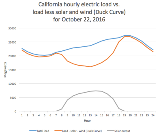
As noted before, a utility system cannot generate more energy than the consumers need. Therefore, the non-solar generation must “take a dip” – which makes the orange curve look somewhat like a duck. This duck-like shape becomes even better visible if one plots similar “total minus solar generation” curves for several consecutive years, as is done in the Fig. \(\PageIndex{2}\).

Figure \(\PageIndex{2}\): Springtime “duck curves” for California for several years, starting from the year 2012. By 2020, the installed solar capacity has increased more than tenfold (plot inspired by videos posted at YouTube by the Vox Group and the US Department of Energy).

What is wrong with the “duck curve”? Well, let’s take a closer look at the curve for the year 2020 in Fig. 11.4. What happens over the seven hours between 2 p.m. and 9 p.m.? The sunlight generation dies out completely, and the demand reaches its evening maximum – the generation has to be ramped up by about 15 GW. And who is going to provide this huge amount of electricity? Well, at the present time (2020) this burden lies overwhelmingly on “peakers”. They are aided by power drawn from energy storage devices, for example, pumped storage power plants – but currently, they are able to provide only a fraction of the power needed. In California there are three types of power plants whose output must remain constant or nearly constant because the intensity of the physical processes employed for generating energy cannot be easily varied “up” and “down”. Those three sectors are: nuclear power, hydropower and geothermal generation, with 2.2 GW, 3.2 GW and 1.5 GW of output power, respectively, and a total of 6.9 GW (let’s call it “the baseline generation”). Accordingly, as it follows from the cited data, at about 2 p.m. the overall California utility system needs about 5 GW generated by burning fossil fuels (mainly natural gas), while by 9 p.m. it already requires about 20 GW from fossil fuels.

Taking into consideration how fast the installation of solar power in California has grown, it can be anticipated that in a few years there will be so much energy from the sun and wind that in the middle of afternoon generation of electricity from natural gas won’t be needed any more. And further installation of new solar and wind farms will already create excess energy in the middle of the day. However, regardless of how much solar energy is deployed, in the evening the state will need 20 GW produced by other means. And this power may be gradually reduced later, but only some time after the next sunrise it won’t be needed any more.

What are those “other means”? – mainly, natural gas peakers. So, even with duplication or even a tripling of installed solar power will not free California’s energy systems from emitting a significant amount of CO₂ making it difficult to achieve its ambitious plans to completely decarbonize the electricity generation. The solution may be to use another zero-emission method of generation, but the only such replacement for natural gas peakers that can be taken into account is wind energy. Yet, the average power of current California’s wind farms is about 1.6 GW (with a total installed power of about 4.5 GW). Hence, to eliminate the gas peakers, the potential of wind farms would have to be increased at least 10 times, which does not seem realistic in a foreseeable future.

California, however, has a very strong resolve to get 100% carbon-neutral by the year 2045. So, the CO₂ emitting peakers must be replaced. By what? There is one more option: by energy-storing devices. The deployment of new solar farms should continue with the same or even faster rate than before. The mid-day “overproduction” should not be curtailed or imported, but instead the energy has to be stored in “rechargeable” devices, from which the power could be later re-drawn. Are there such devices?

What should be the capacity of such a storage facility? Well, the answer is simple: it should be at least the same as the energy provided by the CO₂ emitting sources in California in one 24-hour cycle. One can get a rough estimate of that using a simple model. Based on what was said before, California needs to ramp up fossil-fuel generation from 5 GW at 2 p.m. to 20 GW at 9 p.m., and then the power may be gradually decreased back to 5 GW by the following noon – as illustrated by the simple graph in Fig. 11.5. One can readily carry out a simple integration, from which one gets that the total fossil-fuel energy generated over a 24 hour period is 285 GWh. Please keep in mind that this is only an estimate. When using very simple models, one has to be prepared that the deviations may be significant, 10%, perhaps 20%? But for the considerations that we carry out here, such accuracy is

Figure \(\PageIndex{3}\): A simple graph illustrating the power from fossil fuel generation needed by the California utility system over a 24 hour period. The “triangle” is only a rough approximation of the actual characteristics, the shape of which is rounded and not completely smooth – but such a “triangle” makes the integration straightforward. For the meaning of the red and the green lines, see the text. quite sufficient. We can round up the number we have gotten to 300 GW, it will be easier to remember.

It may be interesting to think of how this picture may change if much more solar generation is added – say, so much that the gas “peakers” won’t be needed in the middle of the day. Then, the “triangle” in Fig. \(\PageIndex{3}\) will start from zero level and perhaps become somewhat narrower – as shown using green lines in Fig. \(\PageIndex{3}\). Then the area encompassed by the blue line corresponds to 200 GWh. Adding more solar will reduce the need for using gas “peakers”, but only by 1/3. Now not 300 GWh of storage capacity will be needed to eliminate the CO₂ emission, but only 200 GWh. Still, a huge capacity!

Is it possible to build a energy storage device of such capacity? Lets look at the largest manufacturer of lithium-ion storage batteries (made primarily for Tesla cars), the Gigafactory 1 plant located in Nevada, not far from the California’s borderline. In 2019 it manufactured batteries of an overall capacity of 35 GWh, and its target capacity planned to be reached by the middle of the current decade is 150 GWh/year. Thus, the creation of storage batteries needed for reaching a total decarbonization of California’s utility lies completely in the capabilities of todays industry. The cost will be astronomical – but there is an old truth: it’s better to pay than to regret later.

Lithium-ion batteries represent only one of several existing technologies that can be employed for storing energy at a level needed by a carbonneutral utility system. On overview of such technologies – existing, as well of emerging – is presented in the following Sections.